Stratégie de suivi des tendances des bénéfices multicouches à moyenne mobile dynamique à indice variable


Date de création: 2025-09-10 11:14:13 Dernière modification: 2025-11-21 11:55:25
Copier: 0 Nombre de clics: 29
2
Suivre
319
Abonnés

Stratégie de suivi des tendances des bénéfices multicouches à moyenne mobile dynamique à indice variable

Aperçu

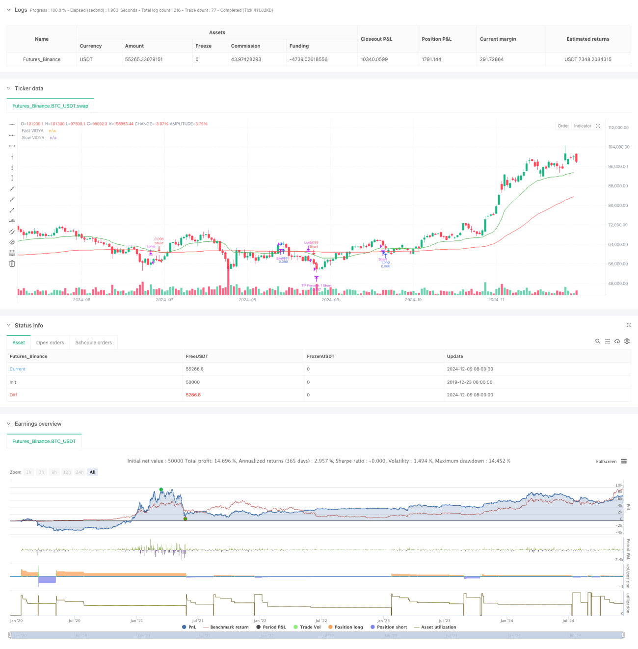
Cette stratégie est un système de suivi de tendance combinant les indices des moyennes dynamiques des variables (VIDYA) et les bandes de Bollinger (Bollinger Bands), tout en intégrant un mécanisme de blocage à plusieurs niveaux. Contrairement aux stratégies de tendance traditionnelles, le système utilise une méthode de profit plus adaptative, distinguant les positions ouvertes par une référence unique à l’ATR et un objectif en pourcentage. Son innovation réside dans l’utilisation d’une méthode de blocage dynamique à plusieurs niveaux, en particulier la multiplication des pourcentages plus radicale pour les transactions à vide.

Principe de stratégie

Le cœur de la stratégie est d’analyser les tendances des prix en utilisant deux indicateurs Vidya, rapide et lent, tout en tenant compte de la volatilité du marché. La formule de calcul de l’indicateur Vidya est: Le facteur d’aplatissement (α) = 2/ (cycle + 1) Vidya (t) = α * k * prix (t) + (1 - α * k) * Vidya (t-1) où k est l’oscillateur dynamique de Chand (MO)

Les bandes de Brin comme filtres de fréquence: La ligne de démarrage = MA + (K * écart-type) La voie inférieure = MA - (K * écart type)

Conditions d’entrée :

  • Coup de tête: le prix a dépassé le Vidya lent et le Vidya rapide a tendance à la hausse, tandis que le prix a dépassé le Brin et s’est mis sur la voie
  • Blank: Le prix est tombé en dessous du Vidya lent et le Vidya rapide a tendance à la baisse, tandis que le prix est tombé en dessous de la bande de Brin

Les dispositifs d’arrêt multicouches comprennent:

  1. Arrêt basé sur ATR
  2. Pourcentage d’arrêt
  3. Le trading à vide utilise des multiplicateurs pour augmenter le taux de stop-loss

Avantages stratégiques

  1. Adaptation dynamique: l’indicateur Vidya s’adapte automatiquement aux fluctuations du marché et est plus sensible que les moyennes traditionnelles
  2. Gestion des risques: un mécanisme de blocage à plusieurs niveaux permet de bloquer les bénéfices à différents niveaux de prix
  3. Traitement différentiel: une stratégie de coupe différente pour les positions ouvertes, plus conforme aux caractéristiques du marché
  4. Filtrage de la fréquence d’oscillation: l’utilisation de la bande Brin peut filtrer les faux signaux de rupture
  5. Flexibilité des paramètres: les paramètres peuvent être ajustés en fonction des différentes conditions du marché

Risque stratégique

  1. Risque de choc: Faux signaux sur le marché horizontal
  2. Effets des points de glissement: plusieurs arrêts peuvent entraîner un écart de prix d’exécution en raison des points de glissement
  3. Paramètres dépendants: les paramètres peuvent nécessiter des ajustements fréquents selon les conditions du marché
  4. Complexité du système: les mécanismes d’arrêt à plusieurs niveaux augmentent la complexité de la stratégie
  5. Pressions sur la gestion des fonds: plusieurs fermetures de positions peuvent entraîner une difficulté accrue de gestion des positions

Orientation de l’optimisation de la stratégie

  1. Ajustement dynamique des paramètres: un système de paramètres adaptatifs peut être développé pour s’adapter automatiquement aux conditions du marché
  2. Identification de l’environnement de marché: ajout d’un module de jugement de l’environnement de marché, utilisant différents paramètres dans différentes conditions de marché
  3. Optimisation de l’arrêt des pertes: augmentation des mécanismes d’arrêt des pertes dynamiques et amélioration de la capacité de contrôle des risques
  4. Filtrage du signal: augmentation des indicateurs auxiliaires tels que le volume de trafic, amélioration de la fiabilité du signal
  5. Gestion des positions: développer des algorithmes de répartition des positions plus intelligents

Résumer

La stratégie crée un système complet de suivi des tendances en combinant l’adaptation dynamique de l’indicateur VIDYA et la fonction de filtrage de la volatilité de la bande de Brin. Un mécanisme de freinage à plusieurs niveaux et un traitement multicouche différencié lui confèrent une bonne rentabilité et une bonne maîtrise des risques. Cependant, les utilisateurs doivent être attentifs aux changements de l’environnement du marché, ajuster les paramètres en temps opportun et mettre en place un système de gestion de fonds bien développé.

Code source de la stratégie
/*backtest
start: 2025-01-01 00:00:00
end: 2025-09-08 08:00:00
period: 1d
basePeriod: 1d
exchanges: [{"eid":"Futures_Binance","currency":"ETH_USDT","balance":500000}]
*/

// This source code is subject to the terms of the Mozilla Public License 2.0 at https://mozilla.org/MPL/2.0/
// © PresentTrading

// This strategy, "VIDYA ProTrend Multi-Tier Profit," is a trend-following system that utilizes fast and slow VIDYA indicators 
// to identify entry and exit points based on the direction and strength of the trend. 
// It incorporates Bollinger Bands as a volatility filter and features a multi-step take profit mechanism, 
// with adjustable ATR-based and percentage-based profit targets for both long and short positions. 
// The strategy allows for more aggressive take profit settings for short trades, making it adaptable to varying market conditions.

//@version=5
strategy("VIDYA ProTrend Multi-Tier Profit", overlay=true)


// User-defined inputs
tradeDirection = input.string(title="Trading Direction", defval="Both", options=["Long", "Short", "Both"])
fastVidyaLength = input.int(10, title="Fast VIDYA Length", minval=1)
slowVidyaLength = input.int(30, title="Slow VIDYA Length", minval=1)
minSlopeThreshold = input.float(0.05, title="Minimum VIDYA Slope Threshold", step=0.01)

// Bollinger Bands Inputs
bbLength = input.int(20, title="Bollinger Bands Length", minval=1)
bbMultiplier = input.float(1.0, title="Bollinger Bands Multiplier", step=0.1)

// Multi-Step Take Profit Settings
group_tp = "Multi-Step Take Profit"
useMultiStepTP = input.bool(true, title="Enable Multi-Step Take Profit", group=group_tp)
tp_direction = input.string(title="Take Profit Direction", defval="Both", options=["Long", "Short", "Both"], group=group_tp)
atrLengthTP =  input.int(14, title="ATR Length", group=group_tp)


// ATR-based Take Profit Steps
atrMultiplierTP1 = input.float(2.618, title="ATR Multiplier for TP 1", group=group_tp)
atrMultiplierTP2 = input.float(5.0, title="ATR Multiplier for TP 2", group=group_tp)
atrMultiplierTP3 = input.float(10.0, title="ATR Multiplier for TP 3", group=group_tp)

// Short Position Multiplier for Take Profit Percentages
shortTPPercentMultiplier = input.float(1.5, title="Short TP Percent Multiplier", group=group_tp)

// Percentage-based Take Profit Steps (Long)
tp_level_percent1 = input.float(title="Take Profit Level 1 (%)", defval=3.0, group=group_tp)
tp_level_percent2 = input.float(title="Take Profit Level 2 (%)", defval=8.0, group=group_tp)
tp_level_percent3 = input.float(title="Take Profit Level 3 (%)", defval=17.0, group=group_tp)

// Percentage-based Take Profit Allocation (Long)
tp_percent1 = input.float(title="Take Profit Percent 1 (%)", defval=12.0, group=group_tp)
tp_percent2 = input.float(title="Take Profit Percent 2 (%)", defval=8.0, group=group_tp)
tp_percent3 = input.float(title="Take Profit Percent 3 (%)", defval=10.0, group=group_tp)

// ATR-based Take Profit Percent Allocation (Long)
tp_percentATR1 = input.float(title="ATR TP Percent 1 (%)", defval=10.0, group=group_tp)
tp_percentATR2 = input.float(title="ATR TP Percent 2 (%)", defval=10.0, group=group_tp)
tp_percentATR3 = input.float(title="ATR TP Percent 3 (%)", defval=10.0, group=group_tp)

// Short position percentage allocations using the multiplier
tp_percent1_short = tp_percent1 * shortTPPercentMultiplier
tp_percent2_short = tp_percent2 * shortTPPercentMultiplier
tp_percent3_short = tp_percent3 * shortTPPercentMultiplier

tp_percentATR1_short = tp_percentATR1 * shortTPPercentMultiplier
tp_percentATR2_short = tp_percentATR2 * shortTPPercentMultiplier
tp_percentATR3_short = tp_percentATR3 * shortTPPercentMultiplier

// VIDYA Calculation Function
calcVIDYA(src, length) =>
    alpha = 2 / (length + 1)
    momm = ta.change(src)
    m1 = momm >= 0.0 ? momm : 0.0
    m2 = momm < 0.0 ? -momm : 0.0
    sm1 = math.sum(m1, length)
    sm2 = math.sum(m2, length)
    chandeMO = nz(100 * (sm1 - sm2) / (sm1 + sm2))
    k = math.abs(chandeMO) / 100
    var float vidya = na
    vidya := na(vidya[1]) ? src : (alpha * k * src + (1 - alpha * k) * vidya[1])
    vidya

// Calculate VIDYAs
fastVIDYA = calcVIDYA(close, fastVidyaLength)
slowVIDYA = calcVIDYA(close, slowVidyaLength)

// Bollinger Bands Calculation
[bbUpper, bbBasis, bbLower] = ta.bb(close, bbLength, bbMultiplier)

// Manual Slope Calculation (price difference over time)
calcSlope(current, previous, length) =>
    (current - previous) / length

// Slope of fast and slow VIDYA (comparing current value with value 'length' bars ago)
fastSlope = calcSlope(fastVIDYA, fastVIDYA[fastVidyaLength], fastVidyaLength)
slowSlope = calcSlope(slowVIDYA, slowVIDYA[slowVidyaLength], slowVidyaLength)

// Conditions for long entry with Bollinger Bands filter
longCondition = close > slowVIDYA and fastSlope > slowSlope and fastSlope > minSlopeThreshold and slowSlope > 1/2*minSlopeThreshold and close > bbUpper

// Conditions for short entry with Bollinger Bands filter
shortCondition = close < slowVIDYA and fastSlope < slowSlope and fastSlope < -minSlopeThreshold and slowSlope < -1/2*minSlopeThreshold and close < bbLower

// Exit conditions (opposite crossovers or flat slopes)
exitLongCondition = fastSlope < -minSlopeThreshold and slowSlope < -1/2*minSlopeThreshold or shortCondition
exitShortCondition = fastSlope > minSlopeThreshold and slowSlope > 1/2*minSlopeThreshold or longCondition

// Entry and Exit logic with trading direction
if (longCondition) and (strategy.position_size == 0) and (tradeDirection == "Long" or tradeDirection == "Both")
    strategy.order("Long", strategy.long)

if (exitLongCondition) and strategy.position_size > 0 and (tradeDirection == "Long" or tradeDirection == "Both")
    strategy.close("Long")

if (shortCondition) and (strategy.position_size == 0) and (tradeDirection == "Short" or tradeDirection == "Both")
    strategy.order("Short", strategy.short)

if (exitShortCondition) and strategy.position_size < 0 and (tradeDirection == "Short" or tradeDirection == "Both")
    strategy.close("Short")


if useMultiStepTP
    if strategy.position_size > 0 and (tp_direction == "Long" or tp_direction == "Both")
        // ATR-based Take Profit (Long)
        tp_priceATR1_long = strategy.position_avg_price + atrMultiplierTP1 * ta.atr(atrLengthTP)
        tp_priceATR2_long = strategy.position_avg_price + atrMultiplierTP2 * ta.atr(atrLengthTP)
        tp_priceATR3_long = strategy.position_avg_price + atrMultiplierTP3 * ta.atr(atrLengthTP)
        
        // Percentage-based Take Profit (Long)
        tp_pricePercent1_long = strategy.position_avg_price * (1 + tp_level_percent1 / 100)
        tp_pricePercent2_long = strategy.position_avg_price * (1 + tp_level_percent2 / 100)
        tp_pricePercent3_long = strategy.position_avg_price * (1 + tp_level_percent3 / 100)

        // Execute ATR-based exits for Long
        strategy.exit("TP ATR 1 Long", from_entry="Long", qty_percent=tp_percentATR1, limit=tp_priceATR1_long)
        strategy.exit("TP ATR 2 Long", from_entry="Long", qty_percent=tp_percentATR2, limit=tp_priceATR2_long)
        strategy.exit("TP ATR 3 Long", from_entry="Long", qty_percent=tp_percentATR3, limit=tp_priceATR3_long)
        
        // Execute Percentage-based exits for Long
        strategy.exit("TP Percent 1 Long", from_entry="Long", qty_percent=tp_percent1, limit=tp_pricePercent1_long)
        strategy.exit("TP Percent 2 Long", from_entry="Long", qty_percent=tp_percent2, limit=tp_pricePercent2_long)
        strategy.exit("TP Percent 3 Long", from_entry="Long", qty_percent=tp_percent3, limit=tp_pricePercent3_long)

    if strategy.position_size < 0 and (tp_direction == "Short" or tp_direction == "Both")
        // ATR-based Take Profit (Short) - using the same ATR levels as long
        tp_priceATR1_short = strategy.position_avg_price - atrMultiplierTP1 * ta.atr(atrLengthTP)
        tp_priceATR2_short = strategy.position_avg_price - atrMultiplierTP2 * ta.atr(atrLengthTP)
        tp_priceATR3_short = strategy.position_avg_price - atrMultiplierTP3 * ta.atr(atrLengthTP)
        
        // Percentage-based Take Profit (Short) - using the same levels, but more aggressive percentages
        tp_pricePercent1_short = strategy.position_avg_price * (1 - tp_level_percent1 / 100)
        tp_pricePercent2_short = strategy.position_avg_price * (1 - tp_level_percent2 / 100)
        tp_pricePercent3_short = strategy.position_avg_price * (1 - tp_level_percent3 / 100)

        // Execute ATR-based exits for Short (using the percentage multiplier for short)
        strategy.exit("TP ATR 1 Short", from_entry="Short", qty_percent=tp_percentATR1_short, limit=tp_priceATR1_short)
        strategy.exit("TP ATR 2 Short", from_entry="Short", qty_percent=tp_percentATR2_short, limit=tp_priceATR2_short)
        strategy.exit("TP ATR 3 Short", from_entry="Short", qty_percent=tp_percentATR3_short, limit=tp_priceATR3_short)
        
        // Execute Percentage-based exits for Short
        strategy.exit("TP Percent 1 Short", from_entry="Short", qty_percent=tp_percent1_short, limit=tp_pricePercent1_short)
        strategy.exit("TP Percent 2 Short", from_entry="Short", qty_percent=tp_percent2_short, limit=tp_pricePercent2_short)
        strategy.exit("TP Percent 3 Short", from_entry="Short", qty_percent=tp_percent3_short, limit=tp_pricePercent3_short)
// Plot VIDYAs
plot(fastVIDYA, color=color.green, title="Fast VIDYA")
plot(slowVIDYA, color=color.red, title="Slow VIDYA")