概要
多層統計回帰取引戦略は,統計的検証と統合された重量配分機構を組み合わせた3層の線形回帰フレームワークを採用した高度な量化取引システムである.この戦略は,短期,中期,および長期の価格動向を同時に分析し,厳格な統計的有意性テストによって高信頼性の方向性信号を生成し,厳格なリスク管理措置を実施する.戦略の核心は,複数の時間枠の線形回帰分析結果を加重統合し,歴史の遡及検証によって信号品質を保証し,信頼性の動向に応じてポジションサイズを調整することです.
戦略原則
この戦略の核心原理は,多層の統計的線形回帰分析に基づいています.主に以下のいくつかの重要な構成要素が含まれています.
多層帰帰引エンジン戦略: 3つのカスタマイズ可能な時間枠 ((短期/中期/長期) で並行して線形回帰分析を行い,デフォルトは20/50/100周期である.各時間枠の斜率,R平方値,関連する係数などの統計指標を計算して,将来の価格動きを予測する.R平方値,関連する係数,および斜率の絶対値が予測する値を超えた場合にのみ,回帰分析の結果は統計的に有意とみなされる.
信号認証システム: 戦略は,歴史的予測値と実際の価格動向を比較して予測の正確性を評価するための後退検証メカニズムを設計した. 重み付け集積方法を使用して3つの時間枠の信号を統合し,短期,中期,および長期の信号に異なる重みを与えます (<0.4/0.35⁄0.25をデフォルトで). 総合信頼度評価は,統計的強度,層間一致性,および検証の正確性を組み合わせています.
リスク管理機構: 戦略は,シグナル信頼性に応じてポジションサイズを動的に調整する (預設口座資金の50%),最大1日損失制限を設定する (預設12%),その制限に達すると自動的に取引を停止する. 戦略は,外為取引の特性を考慮しながら,点差スライドとパーセントベースの手数料設定も含む.
シグナル生成論理は,統合スコアの絶対値が0.5以上であり,総信頼は既定の値 (デフォルト0.75) よりも高く,短期および中期リターンは統計的に顕著で,毎日の損失制限は触発されていない必要があります. 対照的に高い信頼のシグナルが発生した場合,または毎日の損失制限が触発された場合,戦略は平仓操作を実行します.
戦略的優位性
この戦略は,コードを深く分析することで,以下の顕著な利点があります.
多次元市場分析戦略は,短期,中期,長期の価格動向を同時に分析することで,市場動向を全面的に把握し,単一の時間枠がもたらす一方的な判断を避けることができます.
統計の厳密さ戦略: 厳格な統計的有意性テスト ((R平方値,関連系数,斜率値) を実施し,高品質の帰帰帰分析結果のみが信号生成に使用されることを保証し,偽信号の可能性を大幅に低減した.
ポジション管理に適応する戦略: 信号信託の動向に応じてポジションのサイズを調整し,高信託の場合はポジションを増加させ,低信託の場合はリスクの開口を減少させ,リスクと利益のインテリジェントバランスを実現する.
内部認証システム: 予測の正確さを評価する歴史の裏付けにより,信号の品質に追加的な保障層を提供し,戦略の安定性と信頼性を効果的に向上させる.
全面的なリスク管理: 一日の最大損失制限を設定し,一日の大きな損失を防止し,口座の資金の安全性を保護します. 制限に達すると自動的に取引を停止し,市場条件の改善を待つ.
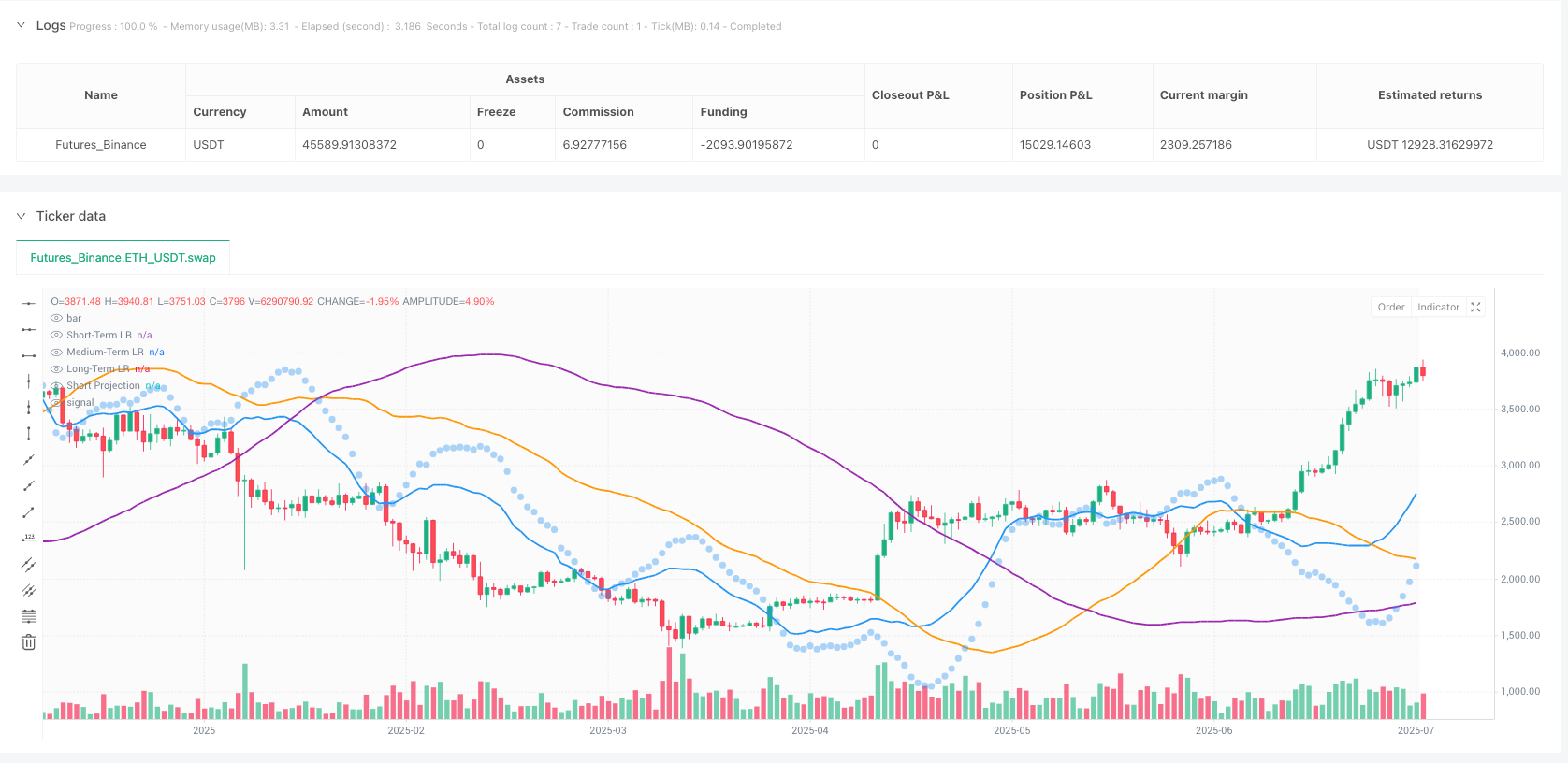
視覚化による意思決定支援戦略は,リアルタイム回帰線グラフ ((3層の異なる色),短期予測マーカー,市場偏向の背景色標識,および総合的な統計データパネル ((R平方指標,検証スコア,損益状況) を提供し,取引決定に直観的なサポートを提供します.
戦略リスク
この戦略の設計は精巧ですが,以下の潜在的なリスクがあります.
パラメータ感度策略は,複数の重要なパラメータ (R平方値,関連系数最小値,斜率値など) に依存し,これらのパラメータの設定は,戦略のパフォーマンスに顕著な影響を及ぼします.不適切なパラメータの設定は,過度取引や重要な信号を逃す可能性があります. 解決策:歴史データを追溯して,パラメータの設定を最適化し,定期的にパラメータの有効性を再評価します.
市場の状況の変化: 高い変動性または突発的なイベントの間,線形回帰の予測能力は著しく低下し,戦略の不良なパフォーマンスを引き起こす可能性があります. 解決策: 市場状態の識別機構を追加し,非線形市場環境で自動的に調整または取引を停止します.
統計の遅れ: 線形回帰分析は本質的に遅滞の指標であり,急激な市場転換で迅速に反応することができない. 解決策: リードインジケーターまたは動力の指標を統合することを考え,市場の転換点に対する戦略の感度を高めること.
オーバーフィットするリスク解決策: 前向きなテストとクロス検証を実施し,戦略の安定性と適応性を確保する.
計算の複雑さ: 戦略の多層回帰分析と統計的検証は,大量の計算リソースを必要とし,高頻度取引環境では実行遅延に直面する可能性があります. 解決策: コード効率を最適化し,より効率的な統計的計算方法を使用することを検討する.
戦略最適化の方向性
この戦略は,以下の方向で最適化できます.
ダイナミックな時間枠への適応:現在の戦略は,固定された短期/中期/長期の時間枠の長さを使用し,市場の変動性に応じてこれらのパラメータを自動的に調整することを考えることができます. 高い変動の市場では時間の枠を短縮し,低い変動の市場では時間の枠を延長し,戦略を異なる市場条件により良く適応させる.
予測モデル強化: 現行の戦略は,線形回帰のみを使用しているが,より複雑なモデルを統合することを考えることができる.例えば,多項式回帰,ARIMA,機械学習モデル (例えば,ランダムフォレスト,サポートベクトルマシンなど) が予測の正確性を向上させる.
市場環境の分類: 市場環境認識モジュールを追加し,トレンド市場と区間振動市場を区別し,異なる市場環境で異なる取引論理とパラメータ設定を採用し,戦略の適応性を向上させる.
検証の最適化:現在のバック検証は,主に短期予測に基づいているが,すべての3つの時間枠に拡張され,ローリングウィンドウのクロス検証などのより複雑な検証方法を実施し,検証の信頼性を高めることができる.
高級リスク管理: ダイナミックなストップ・ローズレベル,波動率調整のポジションサイズ,関連する資産のリスク平価などのより複雑なリスク管理技術を導入し,戦略のリスク調整後の収益をさらに向上させる.
感情と基本的統合: 市場情緒指標や基本的要因,例えば変動率指数,利差差,経済データ発表の影響など,モデルに統合することを検討し,より包括的な取引意思決定の枠組みを作成する.
要約する
多層統計回帰取引戦略は,技術的に高度な,慎重に設計された量化取引システムであり,多層の線形回帰分析と組み合わせた厳密な統計検証とスマートなリスク制御により,取引決定に堅固な数学的基盤を提供します.この戦略の最大の優点は,市場分析の全面的な能力と厳格な統計的手法であり,短期,中期,および長期の価格動向を同時に考慮し,統計的に顕著なテストを行うことで,低品質の信号を効果的にフィルターします.
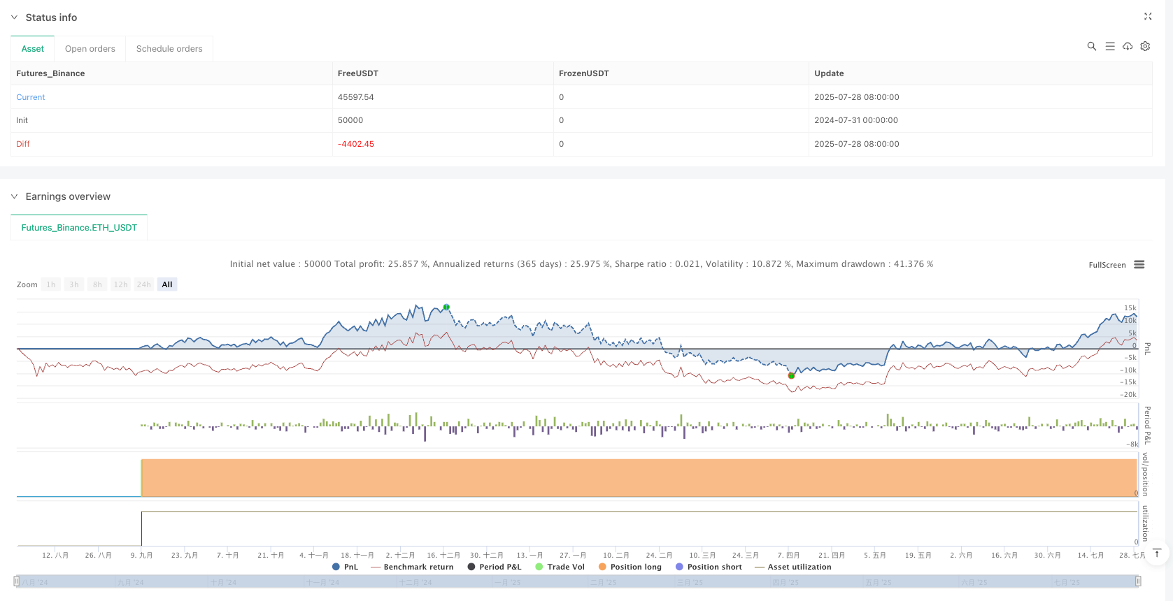
戦略の統合された重量メカニズムと自己適応のポジション管理システムは,信号品質の動向に応じて取引決定とリスクの開口を調整できるようにし,内蔵された後方検証と毎日の損失制限は,追加の安全性を提供します. 完善した可視化インターフェースと統計データパネルは,トレーダーに直感的な意思決定支援ツールを提供します.
この戦略には,パラメータの感受性,市場条件の適応性,統計的遅れなどの潜在的なリスクがあるにもかかわらず,定期的なパラメータ最適化,市場環境の分類,予測モデルの強化などの方向の最適化によって,その安定性と収益性をさらに向上させることができます.全体的に,これは,統計的方法についての知識のあるトレーダーに特に適した,実用的な取引保障と量子金融技術を組み合わせた高度な戦略です.
/*backtest
start: 2024-07-31 00:00:00
end: 2025-07-29 08:00:00
period: 1d
basePeriod: 1d
exchanges: [{"eid":"Futures_Binance","currency":"ETH_USDT"}]
*/

//@version=5
strategy("Multi-Layer Statistical Regression Strategy - Optimized", overlay=true)

// === MULTI-LAYER REGRESSION INPUTS ===
// Linear Regression Layers
lr_short_length = input.int(20, "Short-Term LR Length", minval=10, maxval=50, step=2)
lr_medium_length = input.int(50, "Medium-Term LR Length", minval=30, maxval=100, step=5)
lr_long_length = input.int(100, "Long-Term LR Length", minval=50, maxval=200, step=10)

// === 优化后的统计验证参数 (降低严格程度) ===
min_r_squared = input.float(0.45, "Min R-Squared Threshold", minval=0.2, maxval=0.8, step=0.05)
slope_threshold = input.float(0.00005, "Min Slope Significance", minval=0.00001, maxval=0.001, step=0.00001)
correlation_min = input.float(0.5, "Min Correlation", minval=0.3, maxval=0.8, step=0.05)

// Lookback/Look-Forward Analysis
validation_lookback = input.int(30, "Validation Lookback", minval=10, maxval=60, step=5)
prediction_horizon = input.int(10, "Prediction Horizon", minval=5, maxval=20, step=1)

// Ensemble Weights
weight_short = input.float(0.4, "Short-Term Weight", minval=0.1, maxval=0.6, step=0.1)
weight_medium = input.float(0.35, "Medium-Term Weight", minval=0.1, maxval=0.6, step=0.05)
weight_long = input.float(0.25, "Long-Term Weight", minval=0.1, maxval=0.6, step=0.05)

// === 优化后的风险管理参数 ===
position_size_pct = input.float(50.0, "Position Size %", minval=10.0, maxval=100.0, step=5.0)
max_daily_loss = input.float(12.0, "Max Daily Loss %", minval=5.0, maxval=25.0, step=2.5)
confidence_threshold = input.float(0.55, "Signal Confidence Threshold", minval=0.4, maxval=0.8, step=0.05)

// === 新增:信号强度分级 ===
use_graded_signals = input.bool(true, "Use Graded Signal Strength")
strong_signal_threshold = input.float(0.7, "Strong Signal Threshold", minval=0.6, maxval=0.9, step=0.05)

// === STATISTICAL FUNCTIONS ===
// Calculate Linear Regression with full statistics
linear_regression_stats(src, length) =>
    var float sum_x = 0
    var float sum_y = 0
    var float sum_xy = 0
    var float sum_x2 = 0
    var float sum_y2 = 0

    // Reset sums
    sum_x := 0
    sum_y := 0
    sum_xy := 0
    sum_x2 := 0
    sum_y2 := 0

    // Calculate sums for regression
    for i = 0 to length - 1
        x = i + 1
        y = src[i]
        if not na(y)
            sum_x := sum_x + x
            sum_y := sum_y + y
            sum_xy := sum_xy + x * y
            sum_x2 := sum_x2 + x * x
            sum_y2 := sum_y2 + y * y

    n = length

    // Calculate regression coefficients
    denominator = n * sum_x2 - sum_x * sum_x
    slope = denominator != 0 ? (n * sum_xy - sum_x * sum_y) / denominator : 0
    intercept = (sum_y - slope * sum_x) / n

    // Calculate correlation coefficient (R)
    correlation = (n * sum_xy - sum_x * sum_y) /
                  math.sqrt((n * sum_x2 - sum_x * sum_x) * (n * sum_y2 - sum_y * sum_y))

    // Calculate R-squared
    r_squared = correlation * correlation

    // Current regression value
    current_lr = intercept + slope * n

    // Projected value (look-forward)
    projected_lr = intercept + slope * (n + prediction_horizon)

    [current_lr, slope, r_squared, correlation, projected_lr]

// === 优化后的统计显著性测试 (更灵活) ===
is_statistically_significant(r_squared, correlation, slope_abs, grade = "normal") =>
    if grade == "relaxed"
        r_squared >= (min_r_squared * 0.8) and math.abs(correlation) >= (correlation_min * 0.8) and math.abs(slope_abs) >= (slope_threshold * 0.5)
    else if grade == "strict"
        r_squared >= (min_r_squared * 1.2) and math.abs(correlation) >= (correlation_min * 1.1) and math.abs(slope_abs) >= (slope_threshold * 1.5)
    else
        r_squared >= min_r_squared and math.abs(correlation) >= correlation_min and math.abs(slope_abs) >= slope_threshold

// === MULTI-LAYER REGRESSION ANALYSIS ===
// Short-term layer
[lr_short, slope_short, r2_short, corr_short, proj_short] = linear_regression_stats(close, lr_short_length)
sig_short = is_statistically_significant(r2_short, corr_short, slope_short, "normal")
sig_short_strong = is_statistically_significant(r2_short, corr_short, slope_short, "strict")

// Medium-term layer
[lr_medium, slope_medium, r2_medium, corr_medium, proj_medium] = linear_regression_stats(close, lr_medium_length)
sig_medium = is_statistically_significant(r2_medium, corr_medium, slope_medium, "relaxed")
sig_medium_strong = is_statistically_significant(r2_medium, corr_medium, slope_medium, "normal")

// Long-term layer
[lr_long, slope_long, r2_long, corr_long, proj_long] = linear_regression_stats(close, lr_long_length)
sig_long = is_statistically_significant(r2_long, corr_long, slope_long, "relaxed")

// === LOOKBACK VALIDATION ===
validate_prediction_accuracy() =>
    var array<float> accuracy_scores = array.new<float>()

    if bar_index >= validation_lookback
        historical_slope = (close - close[prediction_horizon]) / prediction_horizon
        predicted_slope = slope_short[prediction_horizon]

        error = math.abs(historical_slope - predicted_slope)
        accuracy = math.max(0, 1 - error * 10000)

        array.push(accuracy_scores, accuracy)
        if array.size(accuracy_scores) > validation_lookback
            array.shift(accuracy_scores)

    array.size(accuracy_scores) > 5 ? array.avg(accuracy_scores) : 0.5

validation_accuracy = validate_prediction_accuracy()

// === 优化后的集成信号生成 ===
// Individual layer signals (directional)
signal_short = sig_short ? (slope_short > 0 ? 1 : -1) : 0
signal_medium = sig_medium ? (slope_medium > 0 ? 1 : -1) : 0
signal_long = sig_long ? (slope_long > 0 ? 1 : -1) : 0

// Weighted ensemble score
ensemble_score = (signal_short * weight_short +
                  signal_medium * weight_medium +
                  signal_long * weight_long)

// === 多级信号置信度计算 ===
// 基础一致性评分
agreement_score = math.abs(signal_short + signal_medium + signal_long) / 3.0

// 统计置信度 (使用加权平均)
stat_confidence = (r2_short * weight_short +
                   r2_medium * weight_medium +
                   r2_long * weight_long)

// 验证置信度
validation_confidence = validation_accuracy

// 整体置信度 (调整权重比例)
overall_confidence = (agreement_score * 0.3 +
                     stat_confidence * 0.5 +
                     validation_confidence * 0.2)

// 信号强度分级
signal_strength = math.abs(ensemble_score)
is_strong_signal = overall_confidence > strong_signal_threshold and (sig_short_strong or sig_medium_strong)

// === POSITION MANAGEMENT ===
trend_direction = ensemble_score > 0 ? 1 : ensemble_score < 0 ? -1 : 0

// 基于信号强度的仓位调整
confidence_multiplier = if use_graded_signals
    if is_strong_signal
        1.0 + (overall_confidence - strong_signal_threshold) * 0.5
    else
        0.7 + (overall_confidence / strong_signal_threshold) * 0.3
else
    overall_confidence > confidence_threshold ? 1.0 : overall_confidence / confidence_threshold

base_position_value = strategy.equity * (position_size_pct / 100)
adjusted_position_value = base_position_value * confidence_multiplier
position_units = adjusted_position_value / close

// Daily loss tracking
var float daily_start_equity = strategy.equity
if ta.change(time("1D"))
    daily_start_equity := strategy.equity

current_daily_loss = daily_start_equity > 0 ? (daily_start_equity - strategy.equity) / daily_start_equity * 100 : 0
halt_trading = current_daily_loss > max_daily_loss

// === 优化后的入场/退出逻辑 ===
// 更灵活的入场条件
long_condition_basic = ensemble_score > 0.2 and overall_confidence > confidence_threshold and sig_short
long_condition_strong = ensemble_score > 0.4 and overall_confidence > strong_signal_threshold and sig_short and sig_medium

short_condition_basic = ensemble_score < -0.2 and overall_confidence > confidence_threshold and sig_short
short_condition_strong = ensemble_score < -0.4 and overall_confidence > strong_signal_threshold and sig_short and sig_medium

// 入场信号生成
long_signal = use_graded_signals ? (long_condition_strong or long_condition_basic) : long_condition_strong
short_signal = use_graded_signals ? (short_condition_strong or short_condition_basic) : short_condition_strong

// 策略执行
if long_signal and not halt_trading and strategy.position_size <= 0
    signal_type = long_condition_strong ? "Strong Long" : "Basic Long"
    strategy.entry("Long", strategy.long, qty=position_units,
                   comment=signal_type + ": " + str.tostring(overall_confidence, "#.##"))

if short_signal and not halt_trading and strategy.position_size >= 0
    signal_type = short_condition_strong ? "Strong Short" : "Basic Short"
    strategy.entry("Short", strategy.short, qty=position_units,
                   comment=signal_type + ": " + str.tostring(overall_confidence, "#.##"))

// 降低初始化门槛
if strategy.position_size == 0 and not halt_trading and barstate.isconfirmed
    if ensemble_score > 0.15 and overall_confidence > (confidence_threshold * 0.8)
        strategy.entry("InitLong", strategy.long, qty=position_units * 0.8, comment="Init Long")
    else if ensemble_score < -0.15 and overall_confidence > (confidence_threshold * 0.8)
        strategy.entry("InitShort", strategy.short, qty=position_units * 0.8, comment="Init Short")

// Emergency exit
if halt_trading and strategy.position_size != 0
    strategy.close_all(comment="Daily Loss Limit")

// === 增强的可视化 ===
// Plot regression lines with transparency based on significance
plot(lr_short, "Short-Term LR", color=sig_short_strong ? color.blue : color.new(color.blue, 50), linewidth=2)
plot(lr_medium, "Medium-Term LR", color=sig_medium_strong ? color.orange : color.new(color.orange, 50), linewidth=2)
plot(lr_long, "Long-Term LR", color=color.new(color.purple, 30), linewidth=1)

// Background with graded confidence
bg_color = if overall_confidence > strong_signal_threshold
    ensemble_score > 0 ? color.new(color.green, 85) : color.new(color.red, 85)
else if overall_confidence > confidence_threshold
    ensemble_score > 0 ? color.new(color.green, 92) : color.new(color.red, 92)
else
    color.new(color.gray, 97)

bgcolor(bg_color)

// Enhanced signal markers
plotshape(long_condition_strong, "Strong Long", shape.triangleup, location.belowbar,
          color=color.green, size=size.large)
plotshape(long_condition_basic and not long_condition_strong, "Basic Long", shape.triangleup, location.belowbar,
          color=color.new(color.green, 40), size=size.small)

plotshape(short_condition_strong, "Strong Short", shape.triangledown, location.abovebar,
          color=color.red, size=size.large)
plotshape(short_condition_basic and not short_condition_strong, "Basic Short", shape.triangledown, location.abovebar,
          color=color.new(color.red, 40), size=size.small)