Rock Solid Turtle 전략

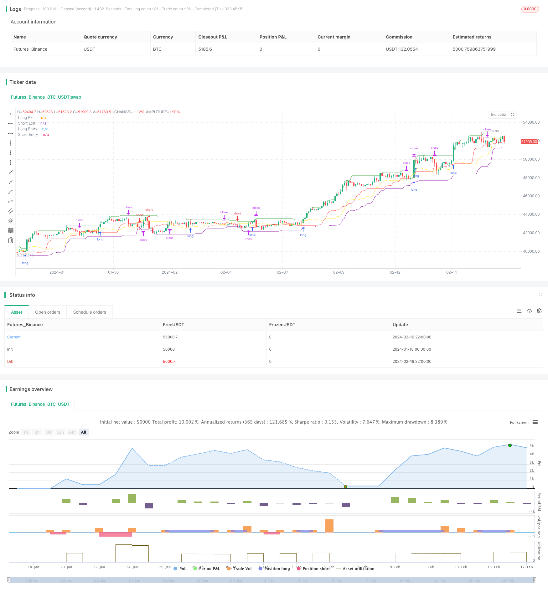
/*backtest
start: 2024-01-18 00:00:00
end: 2024-02-17 00:00:00
period: 2h
basePeriod: 15m
exchanges: [{"eid":"Futures_Binance","currency":"BTC_USDT"}]
*/

//@version=3
strategy("Real Turtle", shorttitle = "Real Turtle", overlay=true, pyramiding=1, default_qty_type= strategy.percent_of_equity,calc_on_order_fills=false, slippage=25,commission_type=strategy.commission.percent,commission_value=0.075)
//////////////////////////////////////////////////////////////////////
// Testing Start dates
testStartYear = input(2016, "Backtest Start Year")
testStartMonth = input(1, "Backtest Start Month")
testStartDay = input(1, "Backtest Start Day")
testPeriodStart = timestamp(testStartYear,testStartMonth,testStartDay,0,0)
//Stop date if you want to use a specific range of dates
testStopYear = input(2030, "Backtest Stop Year")
testStopMonth = input(12, "Backtest Stop Month")
testStopDay = input(30, "Backtest Stop Day")
testPeriodStop = timestamp(testStopYear,testStopMonth,testStopDay,0,0)

// A switch to control background coloring of the test period
// Use if using a specific date range
testPeriodBackground = input(title="Color Background?", type=bool, defval=false)
testPeriodBackgroundColor = testPeriodBackground and (time >= testPeriodStart) and (time <= testPeriodStop) ? #00FF00 : na
bgcolor(testPeriodBackgroundColor, transp=97)

testPeriod() => true
// Component Code Stop
//////////////////////////////////////////////////////////////////////

//How many candles we want to determine our position entry
enterTrade = input(20, minval=1, title="Entry Channel Length")
//How many candles we want ot determine our position exit
exitTrade = input(10, minval=1, title="Exit Channel Length")

//True Range EMA Length
trLength = input(13, minval=1, title="True Range Length")
//Go all in on every trade
allIn = input(false, title="Use whole position on every trade")
dRisk = input(2, "Use Desired Risk %")
//How much of emaTR to use for TS offset
multiEmaTR = input(2, "Desired multiple of ema Tr (N)")
//absolute value (highest high of of this many candles - lowest high of this many candles) . This is used if we want to change our timeframe to a higher timeframe otherwise just works like grabbing high o r low of a candle
//True range is calculated as just high - low. Technically this should be a little more complicated but with 24/7 nature of crypto markets high-low is fine.
trueRange = max(high - low, max(high - close[1], close[1] - low))
//Creates an EMA of the true range by our custom length
emaTR = ema(trueRange, trLength)
//Highest high of how many candles back we want to look as specified in entry channel for long
longEntry = highest(enterTrade)
//loweest low of how many candles back we want to look as specified in exit channel for long
exitLong = lowest(exitTrade)
//lowest low of how many candles back want to look as specified in entry channel for short
shortEntry = lowest(enterTrade)
//lowest low of how many candles back want to look as specified in exit channel for short
exitShort = highest(exitTrade)
//plots the longEntry as a green line
plot(longEntry[1], title="Long Entry",color=green)
//plots the short entry as a purple line
plot(shortEntry[1], title="Short Entry",color=purple)

howFar = barssince(strategy.position_size == 0)
actualLExit = strategy.position_size > 0 ? strategy.position_avg_price - (emaTR[howFar] * multiEmaTR) : longEntry - (emaTR * multiEmaTR)
actualLExit2 = actualLExit > exitLong ? actualLExit : exitLong
actualSExit = strategy.position_size < 0 ? strategy.position_avg_price + (emaTR[howFar] * multiEmaTR) : shortEntry + (emaTR * multiEmaTR)
actualSExit2 = actualSExit < exitShort ? actualSExit : exitShort

//plots the long exit as a red line
plot(actualLExit2[1], title="Long Exit",color=red)
//plots the short exit as a blue line
plot(actualSExit2[1], title="Short Exit",color=yellow)


//Stop loss in ticks
SLLong =(emaTR * multiEmaTR)/ syminfo.mintick
SLShort = (emaTR * multiEmaTR)/ syminfo.mintick


//Calculate our potential loss as a whole percentage number. Example 1 instead of 0.01 for 1% loss. We have to convert back from ticks to whole value, then divided by close
PLLong = ((SLLong * syminfo.mintick) * 100) / longEntry
PLShort = ((SLShort * syminfo.mintick) * 100) / shortEntry
//Calculate our risk by taking our desired risk / potential loss. Then multiple by our equity to get position size. we divide by close because we are using percentage size of equity for quantity in this script as not actual size.
//we then floor the value. which is just to say we round down so instead of say 201.54 we would just input 201 as TV only supports whole integers for quantity.
qtyLong = floor(((dRisk / PLLong) * strategy.equity) /longEntry )
qtyShort = floor(((dRisk / PLShort) * strategy.equity) /shortEntry )
qtyLong2 = allIn ? 100 : qtyLong
qtyShort2 = allIn ? 100 : qtyShort
//Only open long or short positions if we are inside the test period specified earlier
if testPeriod()
    //Open a stop market order at our long entry price and keep it there at the quantity specified. This order is updated/changed on each new candlestick until a position is opened
    strategy.entry("long", strategy.long, stop = longEntry, qty = qtyLong2) 
    //sets up or stop loss order by price specified in our actualLExit2 variable
    strategy.exit("Stoploss-Long", "long", stop=actualLExit2)
    
     //Open a stop market order at our short entry price and keep it there at the quantity specified. This order is updated/changed on each new candlestick until a position is opened
    strategy.entry("short", strategy.short, stop = shortEntry, qty = qtyShort2)
    //sets up or stop loss order by price specified in our actualLExit2 variable
    strategy.exit("Stoploss-Short", "short", stop=actualSExit2)