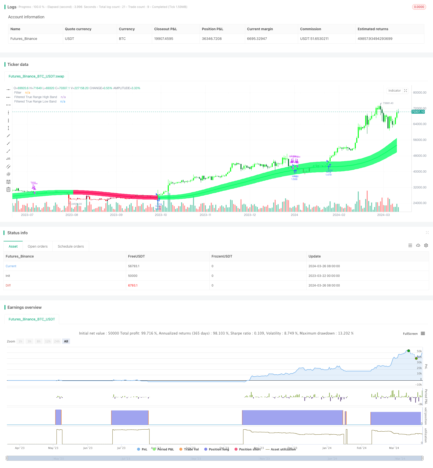
개요
고스 채널 자조선 전략은 고스 파동 기술을 이용한 자조선 전략이다. 이 전략은 존 에렐러스가 제시한 고스 파동 이론에 기초하여 가격 데이터에 대한 여러 지수 이동 평균을 계산하여 부드럽고 적응 가능한 거래 신호를 생성한다. 이 전략의 핵심은 동적으로 조정된 가격 통로를 구성하는 것이며, 상하 궤도는 고스 파동 이후의 가격을 더하여 실제 파동의 폭을 줄이는 것이다.
전략 원칙
고스 통로 자체 적응은 다음과 같다:
- 가격의 고스값을 계산한다. 사용자 설정된 샘플링 주기와 극점 수에 따라 베타와 알파 파라미터를 계산하고, 가격 데이터를 단계적으로 고스값을 계산하여 평형 처리된 가격 순서를 얻는다.
- 실제 변동의 진폭의 고스톤 파동값을 계산한다. 가격의 실제 변동의 진폭에 대해 동일한 고스톤 파동 처리를 하여 부드러운 변동의 진폭 순서를 얻는다.
- 고스 통로를 구성한다. 고스 스 파동 이후의 가격으로 중궤도로, 상궤도는 중궤도로 더한 실제 진동폭과 사용자가 설정한 배수의 곱셈을 하고, 하궤도는 중궤도로 이 값을 어, 동적 통로를 형성한다.
- 거래 신호를 생성한다. 가격이 상향으로 채널을 돌파할 때, 구매 신호를 생성한다. 가격이 하향으로 채널을 돌파할 때, 판매 신호를 생성한다.
- 시간대 파라미터를 도입한다. 사용자는 전략 실행의 시작 및 종료 시간을 설정할 수 있다. 이 시간대 내에서 전략은 거래 신호에 따라 동작한다.
우위 분석
고스 통로의 적응형 평행선 전략은 다음과 같은 장점을 가지고 있다:
- 자기 적응력이 강하다. 전략은 동적으로 조정되는 매개 변수를 채택하고, 다양한 시장 상태와 거래 품종에 적응할 수 있으며, 수동으로 자주调试할 필요가 없다.
- 트렌드 추적성이 좋다. 가격 통로를 구축함으로써, 전략은 시장 추세를 더 잘 포착하고 따라갈 수 있으며, 흔들리는 시장에서 가짜 신호를 효과적으로 피할 수 있다.
- 부드러움: 고스피로파 기술을 사용하여 가격 데이터를 여러 번 부드럽게 처리하여 대부분의 시장 소음을 제거하여 거래 신호를 더 신뢰할 수 있습니다.
- 유연성이 높습니다. 사용자는 필요에 따라 정책 매개 변수, 예를 들어 샘플링 주기, 극점 수, 파동 배수 등을 조정하여 정책 성능을 최적화 할 수 있습니다.
- 실용성이 강하다. 시간영역 파라미터를 도입하여 정책이 지정된 시간 범위에서 실행될 수 있도록 하여 실내 적용과 재검토 연구를 편리하게 한다.
위험 분석
고스 통로 적응형 일률적 전략은 장점이 있지만 위험도 있습니다.
- 매개 변수 설정 위험. 부적절한 매개 변수 설정은 전략의 실패 또는 부적절한 성능을 초래할 수 있으므로 실제 응용에서 반복적으로 테스트 및 최적화가 필요합니다.
- 급격한 사건의 위험. 일부 급격한 중대한 사건에 대응할 때, 전략이 적시에 제대로 대응하지 못하여 손실을 초래할 수 있다.
- 지나치게 잘 맞는 위험. 만약 변수가 너무 잘 맞게 설정되면, 전략이 미래의 성능이 좋지 않을 수 있으며, 샘플 내부와 외부의 성능을 고려해야 한다.
- 경매 위험. 이 전략은 주로 추세 시장에 적용되며, 불안정한 시장에서 자주 거래하면 큰 경매 위험에 직면할 수 있다.
최적화 방향
고스 통로의 일률적 전략에 대한 최적화 방향은 다음과 같습니다.
- 동적 변수 최적화. 기계 학습과 같은 기술을 도입하여 전략 변수의 자동 최적화 및 동적 조정, 적응력을 향상시킵니다.
- 다인자 융합: 다른 유효한 기술 지표 또는 요소를 고스 통로와 결합하여 보다 안정적인 거래 신호를 형성한다.
- 포지션 관리를 최적화한다. 전략의 기초에 합리적인 포지션 관리와 자금 관리 규칙을 추가하고, 철회 및 위험을 통제한다.
- 다중 품종 협동 전략이 여러 가지 다른 거래 품종으로 확장되어 자산配置 및 연관성 분석을 통해 위험을 분산
요약하다
고스 채널 자기 적응 평행 전략은 고스 스 파동과 자기 적응 파라미터에 기반한 양적 거래 전략으로, 동적으로 가격 채널을 구성하여 부드럽고 신뢰할 수 있는 거래 신호를 생성한다. 전략은 자기 적응성이 강하고, 트렌드 추적성이 좋고, 유연성이 높고, 유연성이 강하며, 실용성이 강하지만, 동시에 파라미터 설정, 갑작스러운 사건, 과잉 적합성 및 스쿼리 등의 위험에 직면한다.
전략 소스 코드
/*backtest
start: 2023-03-22 00:00:00
end: 2024-03-27 00:00:00
period: 1d
basePeriod: 1h
exchanges: [{"eid":"Futures_Binance","currency":"BTC_USDT"}]
*/

//@version=4
strategy(title="Gaussian Channel Strategy v1.0", overlay=true, calc_on_every_tick=false, initial_capital=10000, default_qty_type=strategy.percent_of_equity, default_qty_value=100, commission_type=strategy.commission.percent, commission_value=0.1)

// Date condition inputs
startDate = input(title="Date Start", type=input.time, defval=timestamp("1 Jan 2018 00:00 +0000"), group="Dates")
endDate = input(title="Date End", type=input.time, defval=timestamp("31 Dec 2060 23:59 +0000"), group="Dates")
timeCondition = true

// This study is an experiment utilizing the Ehlers Gaussian Filter technique combined with lag reduction techniques and true range to analyze trend activity.
// Gaussian filters, as Ehlers explains it, are simply exponential moving averages applied multiple times.
// First, beta and alpha are calculated based on the sampling period and number of poles specified. The maximum number of poles available in this script is 9.
// Next, the data being analyzed is given a truncation option for reduced lag, which can be enabled with "Reduced Lag Mode".
// Then the alpha and source values are used to calculate the filter and filtered true range of the dataset.
// Filtered true range with a specified multiplier is then added to and subtracted from the filter, generating a channel.
// Lastly, a one pole filter with a N pole alpha is averaged with the filter to generate a faster filter, which can be enabled with "Fast Response Mode".

//Custom bar colors are included.

//Note: Both the sampling period and number of poles directly affect how much lag the indicator has, and how smooth the output is.
//      Larger inputs will result in smoother outputs with increased lag, and smaller inputs will have noisier outputs with reduced lag.
//      For the best results, I recommend not setting the sampling period any lower than the number of poles + 1. Going lower truncates the equation.

//-----------------------------------------------------------------------------------------------------------------------------------------------------------------
//Updates:
// Huge shoutout to @e2e4mfck for taking the time to improve the calculation method!
// -> migrated to v4
// -> pi is now calculated using trig identities rather than being explicitly defined.
// -> The filter calculations are now organized into functions rather than being individually defined.
// -> Revamped color scheme.

//-----------------------------------------------------------------------------------------------------------------------------------------------------------------
//Functions - courtesy of @e2e4mfck
//-----------------------------------------------------------------------------------------------------------------------------------------------------------------

//Filter function
f_filt9x (_a, _s, _i) =>
    int _m2 = 0, int _m3 = 0, int _m4 = 0, int _m5 = 0, int _m6 = 0,
    int _m7 = 0, int _m8 = 0, int _m9 = 0, float _f = .0, _x = (1 - _a)
    // Weights.
    // Initial weight _m1 is a pole number and equal to _i
    _m2 := _i == 9 ? 36  : _i == 8 ? 28 : _i == 7 ? 21 : _i == 6 ? 15 : _i == 5 ? 10 : _i == 4 ? 6 : _i == 3 ? 3 : _i == 2 ? 1 : 0
    _m3 := _i == 9 ? 84  : _i == 8 ? 56 : _i == 7 ? 35 : _i == 6 ? 20 : _i == 5 ? 10 : _i == 4 ? 4 : _i == 3 ? 1 : 0
    _m4 := _i == 9 ? 126 : _i == 8 ? 70 : _i == 7 ? 35 : _i == 6 ? 15 : _i == 5 ? 5  : _i == 4 ? 1 : 0
    _m5 := _i == 9 ? 126 : _i == 8 ? 56 : _i == 7 ? 21 : _i == 6 ? 6  : _i == 5 ? 1  : 0
    _m6 := _i == 9 ? 84  : _i == 8 ? 28 : _i == 7 ? 7  : _i == 6 ? 1  : 0
    _m7 := _i == 9 ? 36  : _i == 8 ? 8  : _i == 7 ? 1  : 0
    _m8 := _i == 9 ? 9   : _i == 8 ? 1  : 0
    _m9 := _i == 9 ? 1   : 0
    // filter
    _f :=   pow(_a, _i) * nz(_s) +
      _i  *     _x      * nz(_f[1])      - (_i >= 2 ?
      _m2 * pow(_x, 2)  * nz(_f[2]) : 0) + (_i >= 3 ?
      _m3 * pow(_x, 3)  * nz(_f[3]) : 0) - (_i >= 4 ?
      _m4 * pow(_x, 4)  * nz(_f[4]) : 0) + (_i >= 5 ?
      _m5 * pow(_x, 5)  * nz(_f[5]) : 0) - (_i >= 6 ?
      _m6 * pow(_x, 6)  * nz(_f[6]) : 0) + (_i >= 7 ?
      _m7 * pow(_x, 7)  * nz(_f[7]) : 0) - (_i >= 8 ?
      _m8 * pow(_x, 8)  * nz(_f[8]) : 0) + (_i == 9 ?
      _m9 * pow(_x, 9)  * nz(_f[9]) : 0)

//9 var declaration fun
f_pole (_a, _s, _i) =>
    _f1 =            f_filt9x(_a, _s, 1),      _f2 = (_i >= 2 ? f_filt9x(_a, _s, 2) : 0), _f3 = (_i >= 3 ? f_filt9x(_a, _s, 3) : 0)
    _f4 = (_i >= 4 ? f_filt9x(_a, _s, 4) : 0), _f5 = (_i >= 5 ? f_filt9x(_a, _s, 5) : 0), _f6 = (_i >= 6 ? f_filt9x(_a, _s, 6) : 0)
    _f7 = (_i >= 2 ? f_filt9x(_a, _s, 7) : 0), _f8 = (_i >= 8 ? f_filt9x(_a, _s, 8) : 0), _f9 = (_i == 9 ? f_filt9x(_a, _s, 9) : 0)
    _fn = _i == 1 ? _f1 : _i == 2 ? _f2 : _i == 3 ? _f3 :
      _i == 4     ? _f4 : _i == 5 ? _f5 : _i == 6 ? _f6 :
      _i == 7     ? _f7 : _i == 8 ? _f8 : _i == 9 ? _f9 : na
    [_fn, _f1]

//-----------------------------------------------------------------------------------------------------------------------------------------------------------------
//Inputs
//-----------------------------------------------------------------------------------------------------------------------------------------------------------------

//Source
src = input(defval=hlc3, title="Source")

//Poles
int N = input(defval=4, title="Poles", minval=1, maxval=9)

//Period
int per = input(defval=144, title="Sampling Period", minval=2)

//True Range Multiplier
float mult = input(defval=1.414, title="Filtered True Range Multiplier", minval=0)

//Lag Reduction
bool modeLag  = input(defval=false, title="Reduced Lag Mode")
bool modeFast = input(defval=false, title="Fast Response Mode")

//-----------------------------------------------------------------------------------------------------------------------------------------------------------------
//Definitions
//-----------------------------------------------------------------------------------------------------------------------------------------------------------------

//Beta and Alpha Components
beta  = (1 - cos(4*asin(1)/per)) / (pow(1.414, 2/N) - 1)
alpha = - beta + sqrt(pow(beta, 2) + 2*beta)

//Lag
lag = (per - 1)/(2*N)

//Data
srcdata = modeLag ? src + (src - src[lag]) : src
trdata  = modeLag ? tr(true) + (tr(true) - tr(true)[lag]) : tr(true)

//Filtered Values
[filtn, filt1]     = f_pole(alpha, srcdata, N)
[filtntr, filt1tr] = f_pole(alpha, trdata,  N)

//Lag Reduction
filt   = modeFast ? (filtn + filt1)/2 : filtn
filttr = modeFast ? (filtntr + filt1tr)/2 : filtntr

//Bands
hband = filt + filttr*mult
lband = filt - filttr*mult

// Colors
color1   = #0aff68
color2   = #00752d
color3   = #ff0a5a
color4   = #990032
fcolor   = filt > filt[1] ? #0aff68 : filt < filt[1] ? #ff0a5a : #cccccc
barcolor = (src > src[1]) and (src > filt) and (src < hband) ? #0aff68 : (src > src[1]) and (src >= hband) ? #0aff1b : (src <= src[1]) and (src > filt) ? #00752d :
           (src < src[1]) and (src < filt) and (src > lband) ? #ff0a5a : (src < src[1]) and (src <= lband) ? #ff0a11 : (src >= src[1]) and (src < filt) ? #990032 : #cccccc

//-----------------------------------------------------------------------------------------------------------------------------------------------------------------
//Outputs
//-----------------------------------------------------------------------------------------------------------------------------------------------------------------

//Filter Plot
filtplot = plot(filt, title="Filter", color=fcolor, linewidth=3)

//Band Plots
hbandplot = plot(hband, title="Filtered True Range High Band", color=fcolor)
lbandplot = plot(lband, title="Filtered True Range Low Band", color=fcolor)

//Channel Fill
fill(hbandplot, lbandplot, title="Channel Fill", color=fcolor, transp=80)

//Bar Color
barcolor(barcolor)


longCondition = crossover(close, hband) and timeCondition
closeAllCondition = crossunder(close, hband) and timeCondition

if longCondition
    strategy.entry("long", strategy.long)

if closeAllCondition
    strategy.close("long")