이동평균선, 지지저항선, 거래량에 기반한 고급 진입 조건 전략

1
Follow
1781
Followers
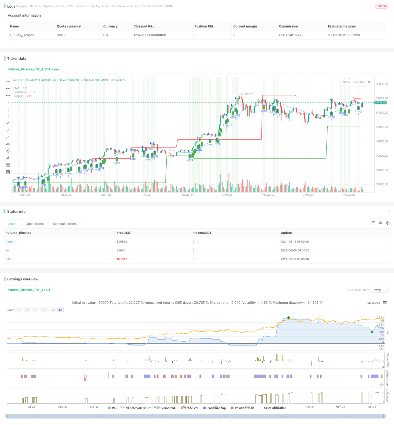
개요
이 전략은 간단한 이동 평균 ((SMA), 지지부진 및 거래량이 증가하는 세 가지 기술 지표를 결합하여 포괄적인 거래 전략을 구성한다. 전략의 주요 아이디어는 가격이 SMA 평균선을 돌파하고 지지부진을 지지하며 거래량이 증가하는 상황에서 거래하며, 위험을 제어하기 위해 중지 조건을 설정한다.
전략 원칙
- 지정된 주기 SMA 평균선, 지지점과 저항점을 계산한다.
- 현재 거래량이 이전 기간보다 증가했는지 판단하십시오.
- 다중 입점 조건: 현재 종료 가격은 이전 주기 종료 가격보다 크고, SMA 평균선과 지지점보다 크며, 가격은 저항점으로부터 일정 거리이며 거래량이 증가한다.
- 공허 입시 조건: 현재 종료 가격은 전주기 종료 가격보다 낮으며 SMA 평균선과 지지점보다 낮으며 가격은 저항점으로부터 일정 거리이며 거래량이 증가한다.
- 손실 조건: 다중 헤드 스톱 가격은 입시 가격으로 곱하기 ((1- 손실 비율), 공허 헤드 스톱 가격은 입시 가격으로 곱하기 ((1+ 손실 비율) <unk>.
우위 분석
- 여러 기술 지표와 결합하여 전략의 신뢰성과 안정성을 높였습니다.
- 가격의 SMA 평균선과 지지부진을 돌파하는 것을 고려하여 트렌드 기회를 더 잘 잡을 수 있습니다.
- 거래량 지표를 도입하여 가격 돌파가 충분한 시장 참여와 함께 이루어지도록 보장하여 신호의 효과를 높였습니다.
- 스톱로스 조건을 설정하여 거래 위험을 효과적으로 통제합니다.
위험 분석
- 저항 지점을 지원하는 계산은 역사적인 데이터에 의존하며, 시장의 큰 변동이 있을 때 유효성을 잃을 수 있다.
- 거래량 지표에 비정상적인 변동이 있을 수 있으며, 이는 잘못된 신호를 발생시킬 수 있다.
- 스톱로스 조건의 설정은 시장의 극단적인 상황에서의 손실을 완전히 피할 수 없습니다.
최적화 방향
- 상대적으로 약한 지수 (RSI) 또는 이동 평균의 종결 분산 (MACD) 과 같은 다른 기술 지표를 도입하는 것을 고려하여 거래 신호의 신뢰성을 추가로 검증하십시오.
- 지원 저항 지점을 계산하는 방법을 최적화하여, 예를 들어, 다른 시장 상황에 적응하기 위해 더 역동적인 방법을 사용합니다.
- 거래량 지표에 대한 부드러운 처리가 비정상적인 변동이 전략에 미치는 영향을 줄여줍니다.
- 이동식 스톱을 사용하거나 시장의 변동에 따라 스톱 퍼센티지를 동적으로 조정하는 등의 최적화된 스톱 조건을 설정합니다.
요약하다
이 전략은 SMA 평균선, 지지부진 및 거래량 지표를 결합하여 포괄적인 거래 전략을 구축한다. 전략의 장점은 트렌드적 기회를 포착하고 거래 위험을 제어하는 데 있다. 그러나 전략에는 시장의 극단적 인 상황에 대한 적응력을 향상시키는 것과 같은 특정 한계가 있습니다.
Source
Pine
Strategy parameters
Related strategies
Comment
All comments (0)
No data
- 1