평균 회귀 볼린저 밴드 달러 비용 평균화 전략

BB DCA EMA SMA
생성 날짜: 2024-12-12 17:17:15 마지막으로 수정됨: 2024-12-12 17:17:15
복사: 2 클릭수: 447
avatar of ChaoZhang ChaoZhang
1
집중하다
1617
수행원

평균 회귀 볼린저 밴드 달러 비용 평균화 전략

개요

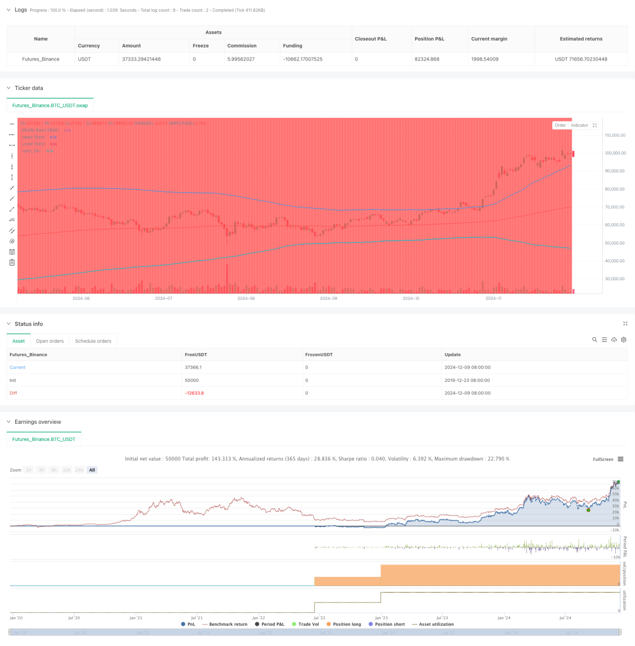
이 전략은 달러 비용 평균법 ((DCA) 과 부린띠 기술 지표를 결합한 지능적인 투자 전략이다. 그것은 가격 회귀 기간 동안 체계적으로 포지션을 구축하여 평균 회귀 원리를 활용하여 투자한다. 이 전략의 핵심은 가격이 부린띠의 궤도를 벗어나면 고정 금액의 구매 작업을 수행하여 시장 조정 기간 동안 더 나은 입시 가격을 얻는다.

전략 원칙

전략의 핵심 원칙은 세 가지 기초에 기반합니다: 1) 달러 비용 평균법, 주기적으로 고정 금액을 투입하여 선택의 위험을 줄이는 것; 2) 평균 회귀 이론, 가격이 결국 역사적 평균 수준으로 돌아간다고 생각하는 것; 3) 부린 띠 지표, 과매도 영역을 식별하기 위해. 가격이 부린 띠 아래로 돌파 할 때 구매 신호를 유발하고, 구매 금액은 설정된 투자 금액을 배분하여 현재 가격을 결정한다. 전략은 200 주기 지수 이동 평균선을 부린 띠의 궤도 중 하나로 사용하고, 표준 차이는 2 이므로 상하 궤도를 정의합니다.

전략적 이점

  1. 선택의 위험을 줄여주기 - 주관적인 판단보다는 체계적인 구매를 통해 인간 오류를 줄여주기
  2. 회수 기회를 잡기 - 가격 초하락 시 자동으로 구매
  3. 유연한 변수 설정 - 다양한 시장 환경에 따라 브린 밴드 변수 및 투자 금액을 조정할 수 있습니다.
  4. 명확한 출전 규칙 - 기술 지표에 기반한 객관적 신호
  5. 자동화 실행 - 인간의 개입 없이 감정적 거래를 피하는 방법

전략적 위험

  1. 평균 회귀 실패 위험 - 트렌드 시장에서 더 많은 가짜 신호가 발생할 수 있습니다.
  2. 자금 관리 위험 - 연속 구매 신호에 대응하기 위해 충분한 자금을 준비해야 합니다.
  3. 매개 변수 최적화 위험 - 과도한 최적화는 전략의 실패로 이어질 수 있습니다.
  4. 시장 환경 의존성 - 급격한 변동성 시장에서 부진할 수 있습니다. 이러한 위험을 관리하기 위해 엄격한 자금 관리 시스템과 정기적으로 전략의 성과를 평가하는 것이 좋습니다.

전략 최적화 방향

  1. 트렌드 필터를 도입하여 강력한 트렌드에서 역동적인 조작을 피하십시오.
  2. 다중 시간 주기 확인 메커니즘을 추가합니다.
  3. 자본 관리 시스템을 최적화하여 변동율에 따라 투자 금액을 조정합니다.
  4. 이득이 되는 결제 메커니즘에 가입하여, 가격이 평균으로 돌아가는 동안 이득이 되는 결제
  5. 다른 기술 지표와 결합하여 신호 신뢰성을 향상시키는 것을 고려하십시오.

요약하다

이것은 기술적 분석과 체계화된 투자방법을 결합한 안정적인 전략이다. 부린을 통해 오버박 기회를 식별하고, 달러 비용 평균법과 함께 위험을 줄인다. 전략의 성공에 핵심은 파라미터의 합리적인 설정과 엄격한 실행 규율에 있다.

전략 소스 코드
/*backtest
start: 2019-12-23 08:00:00
end: 2024-12-10 08:00:00
period: 1d
basePeriod: 1d
exchanges: [{"eid":"Futures_Binance","currency":"BTC_USDT"}]
*/

//@version=5
strategy("DCA Strategy with Mean Reversion and Bollinger Band", overlay=true) // Define the strategy name and set overlay=true to display on the main chart

// Inputs for investment amount and dates
investment_amount = input.float(10000, title="Investment Amount (USD)", tooltip="Amount to be invested in each buy order (in USD)") // Amount to invest in each buy order
open_date = input(timestamp("2024-01-01 00:00:00"), title="Open All Positions On", tooltip="Date when to start opening positions for DCA strategy") // Date to start opening positions
close_date = input(timestamp("2024-08-04 00:00:00"), title="Close All Positions On", tooltip="Date when to close all open positions for DCA strategy") // Date to close all positions

// Bollinger Band parameters
source = input.source(title="Source", defval=close, group="Bollinger Band Parameter", tooltip="The price source to calculate the Bollinger Bands (e.g., closing price)") // Source of price for calculating Bollinger Bands (e.g., closing price)
length = input.int(200, minval=1, title='Period', group="Bollinger Band Parameter", tooltip="Period for the Bollinger Band calculation (e.g., 200-period moving average)") // Period for calculating the Bollinger Bands (e.g., 200-period moving average)
mult = input.float(2, minval=0.1, maxval=50, step=0.1, title='Standard Deviation', group="Bollinger Band Parameter", tooltip="Multiplier for the standard deviation to define the upper and lower bands") // Multiplier for the standard deviation to calculate the upper and lower bands

// Timeframe selection for Bollinger Bands
tf = input.timeframe(title="Bollinger Band Timeframe", defval="240", group="Bollinger Band Parameter", tooltip="The timeframe used to calculate the Bollinger Bands (e.g., 4-hour chart)") // Timeframe for calculating the Bollinger Bands (e.g., 4-hour chart)

// Calculate BB for the chosen timeframe using security
[basis, bb_dev] = request.security(syminfo.tickerid, tf, [ta.ema(source, length), mult * ta.stdev(source, length)]) // Calculate Basis (EMA) and standard deviation for the chosen timeframe
upper = basis + bb_dev // Calculate the Upper Band by adding the standard deviation to the Basis
lower = basis - bb_dev // Calculate the Lower Band by subtracting the standard deviation from the Basis

// Plot Bollinger Bands
plot(basis, color=color.red, title="Middle Band (SMA)") // Plot the middle band (Basis, EMA) in red
plot(upper, color=color.blue, title="Upper Band") // Plot the Upper Band in blue
plot(lower, color=color.blue, title="Lower Band") // Plot the Lower Band in blue
fill(plot(upper), plot(lower), color=color.blue, transp=90) // Fill the area between Upper and Lower Bands with blue color at 90% transparency

// Define buy condition based on Bollinger Band 
buy_condition = ta.crossunder(source, lower) // Define the buy condition when the price crosses under the Lower Band (Mean Reversion strategy)

// Execute buy orders on the Bollinger Band Mean Reversion condition
if (buy_condition ) // Check if the buy condition is true and time is within the open and close date range
    strategy.order("DCA Buy", strategy.long, qty=investment_amount / close) // Execute the buy order with the specified investment amount

// Close all positions on the specified date
if (time >= close_date) // Check if the current time is after the close date
    strategy.close_all() // Close all open positions

// Track the background color state
var color bgColor = na // Initialize a variable to store the background color (set to 'na' initially)

// Update background color based on conditions
if close > upper // If the close price is above the Upper Band
    bgColor := color.red // Set the background color to red
else if close < lower // If the close price is below the Lower Band
    bgColor := color.green // Set the background color to green

// Apply the background color
bgcolor(bgColor, transp=90, title="Background Color Based on Bollinger Bands") // Set the background color based on the determined condition with 90% transparency

// Postscript:
// 1. Once you have set the "Investment Amount (USD)" in the input box, proceed with additional configuration. 
// Go to "Properties" and adjust the "Initial Capital" value by calculating it as "Total Closed Trades" multiplied by "Investment Amount (USD)" 
// to ensure the backtest results are aligned correctly with the actual investment values.
//
// Example:
// Investment Amount (USD) = 100 USD
// Total Closed Trades = 10 
// Initial Capital = 10 x 100 = 1,000 USD

// Investment Amount (USD) = 200 USD
// Total Closed Trades = 24 
// Initial Capital = 24 x 200 = 4,800 USD