
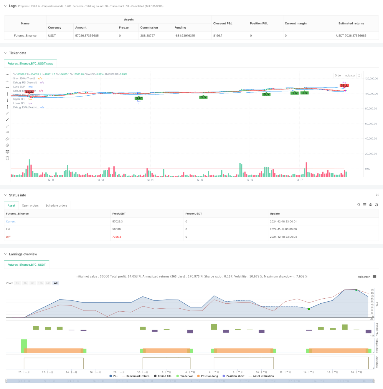
이 전략은 여러 기술 지표가 결합된 통합 거래 시스템으로, 주로 동적으로 시장의 움직임과 추세 변화를 모니터링하여 거래 기회를 잡습니다. 전략은 평평선 시스템 ((EMA), 상대적으로 강한 지표 ((RSI), 이동 평균 수렴 분산 지표 ((MACD), 부린 밴드 ((BB)) 과 같은 여러 지표를 통합하고, 실제 파도 (ATR) 에 기반한 동적 손실 제도를 도입하여 시장의 다차원 분석과 위험을 제어합니다.
이 전략은 여러 계층의 신호 확인 메커니즘을 적용하고 있으며, 주로 다음과 같은 요소들을 포함합니다.
이 전략은 다중 지표 협동으로 비교적 완전한 거래 시스템을 구축한다. 핵심 장점은 다차원적인 신호 확인 메커니즘과 역동적인 위험 제어 시스템이지만, 또한 파라미터 최적화 및 시장 적응성에 주의를 기울여야 한다. 지속적인 최적화 및 조정으로 이 전략은 다양한 시장 환경에서 안정적인 성능을 유지할 것으로 보인다.
/*backtest
start: 2024-11-19 00:00:00
end: 2024-12-19 00:00:00
period: 1h
basePeriod: 1h
exchanges: [{"eid":"Futures_Binance","currency":"BTC_USDT"}]
*/
//@version=5
strategy("XRP/USDT Scalping Strategy", overlay=true)
// Input Parameters
emaShortLength = input.int(7, title="Short EMA Length")
emaLongLength = input.int(14, title="Long EMA Length")
rsiLength = input.int(7, title="RSI Length")
rsiOverbought = input.int(70, title="RSI Overbought Level") // Adjusted to 70 for broader range
rsiOversold = input.int(30, title="RSI Oversold Level") // Adjusted to 30 for broader range
macdFastLength = input.int(12, title="MACD Fast Length")
macdSlowLength = input.int(26, title="MACD Slow Length")
macdSignalLength = input.int(9, title="MACD Signal Length")
bbLength = input.int(20, title="Bollinger Bands Length")
bbStdDev = input.float(2.0, title="Bollinger Bands Standard Deviation") // Adjusted to 2.0 for better signal detection
// EMA Calculation
emaShort = ta.ema(close, emaShortLength)
emaLong = ta.ema(close, emaLongLength)
// RSI Calculation
rsi = ta.rsi(close, rsiLength)
// MACD Calculation
[macdLine, signalLine, _] = ta.macd(close, macdFastLength, macdSlowLength, macdSignalLength)
macdHistogram = macdLine - signalLine
// Bollinger Bands Calculation
basis = ta.sma(close, bbLength)
deviation = ta.stdev(close, bbLength)
bbUpper = basis + (bbStdDev * (deviation > 1e-5 ? deviation : 1e-5)) // Ensure robust Bollinger Band calculation
bbLower = basis - bbStdDev * deviation
// Volume Condition
volCondition = volume > ta.sma(volume, input.int(20, title="Volume SMA Period")) // Dynamic volume filter
// Trend Strength (ADX)
// True Range Calculation
tr = math.max(high - low, math.max(math.abs(high - close[1]), math.abs(low - close[1])))
// Directional Movement
plusDM = high - high[1] > low[1] - low ? math.max(high - high[1], 0) : 0
minusDM = low[1] - low > high - high[1] ? math.max(low[1] - low, 0) : 0
// Smooth Moving Averages
atr_custom = ta.rma(tr, 14)
plusDI = 100 * ta.rma(plusDM, 14) / atr_custom // Correct reference to atr_custom
minusDI = 100 * ta.rma(minusDM, 14) / atr_custom // Correct reference to atr_custom
// ADX Calculation
adx = plusDI + minusDI > 0 ? 100 * ta.rma(math.abs(plusDI - minusDI) / (plusDI + minusDI), 14) : na // Simplified ternary logic for ADX calculation // Prevent division by zero // Prevent division by zero // Final ADX
strongTrend = adx > 25
// Conditions for Buy Signal
emaBullish = emaShort > emaLong
rsiOversoldCondition = rsi < rsiOversold
macdBullishCrossover = ta.crossover(macdLine, signalLine)
priceAtLowerBB = close <= bbLower
buySignal = emaBullish and (rsiOversoldCondition or macdBullishCrossover or priceAtLowerBB) // Relaxed conditions by removing volCondition and strongTrend
// Conditions for Sell Signal
emaBearish = emaShort < emaLong
rsiOverboughtCondition = rsi > rsiOverbought
macdBearishCrossover = ta.crossunder(macdLine, signalLine)
priceAtUpperBB = close >= bbUpper
sellSignal = emaBearish and (rsiOverboughtCondition or macdBearishCrossover or priceAtUpperBB) // Relaxed conditions by removing volCondition and strongTrend
// Plot EMA Lines
trendColor = emaShort > emaLong ? color.green : color.red
plot(emaShort, color=trendColor, title="Short EMA (Trend)") // Simplified color logic
plot(emaLong, color=color.red, title="Long EMA")
// Plot Bollinger Bands
plot(bbUpper, color=color.blue, title="Upper BB")
plot(bbLower, color=color.blue, title="Lower BB")
// Plot Buy and Sell Signals
plot(emaBullish ? 1 : na, color=color.green, linewidth=1, title="Debug: EMA Bullish")
plot(emaBearish ? 1 : na, color=color.red, linewidth=1, title="Debug: EMA Bearish")
plot(rsiOversoldCondition ? 1 : na, color=color.orange, linewidth=1, title="Debug: RSI Oversold")
plot(rsiOverboughtCondition ? 1 : na, color=color.purple, linewidth=1, title="Debug: RSI Overbought")
plotshape(series=buySignal, title="Buy Signal", location=location.belowbar, color=color.green, style=shape.labelup, text="BUY")
plotshape(series=sellSignal, title="Sell Signal", location=location.abovebar, color=color.red, style=shape.labeldown, text="SELL", size=size.small) // Dynamic size for signals
// Strategy Execution with ATR-based Stop Loss and Take Profit
// Reuse atr_custom from earlier calculation
stopLoss = low - (input.float(1.5, title="Stop Loss Multiplier") * atr_custom) // Consider dynamic adjustment based on market conditions // Adjustable stop-loss multiplier
takeProfit = close + (2 * atr_custom)
if (buySignal)
strategy.entry("Buy", strategy.long, stop=stopLoss) // Removed limit to simplify trade execution
if (sellSignal)
strategy.close("Buy")