동적 적응형 다중 시간대 추세 추적 및 충격 반전 복합 전략

ICHIMOKU MACD RSI ATR STOCHASTIC RSI
생성 날짜: 2025-02-20 14:25:14 마지막으로 수정됨: 2025-02-20 14:48:41
복사: 0 클릭수: 339
avatar of ianzeng123 ianzeng123
2
집중하다
319
수행원

동적 적응형 다중 시간대 추세 추적 및 충격 반전 복합 전략 동적 적응형 다중 시간대 추세 추적 및 충격 반전 복합 전략

개요

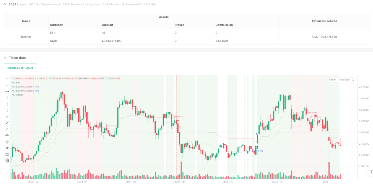
이 전략은 트렌드 추적과 간격 거래를 결합한 복합적인 거래 시스템으로, Ichimoku 클라우드 그래프를 통해 시장 상태를 식별하고, MACD 동력 확인과 RSI 오버 바이 오버 시드 지표를 결합하고, ATR을 사용하여 동적 스톱 로즈 관리를 수행합니다. 이 전략은 트렌드 시장에서 트렌드 기회를 포착하고, 흔들리는 시장에서 역전 기회를 찾으며, 강한 적응력과 유연성을 가지고 있습니다.

전략 원칙

이 전략은 다단계 신호 확인 메커니즘을 사용합니다.

  1. 이치모쿠 클라우드 그래프를 시장 상태를 판단하는 주요 근거로 사용하여, 가격과 클라우드의 위치 관계를 통해 시장이 트렌드 상태인지 흔들리는 상태인지 판단합니다.
  2. 트렌드 시장에서, 가격이 클라우드 위에 있고 RSI>55과 MACD 기둥이 긍정적일 때, 더 많이 입는 것; 가격이 클라우드 아래에 있고 RSI<45과 MACD 기둥이 부정일 때, 입는 것
  3. 흔들리는 시장에서 RSI <30과 임의의 RSI <20일 때, 더 많은 기회를 찾습니다. RSI>70과 임의의 RSI>80일 때, 더 많은 기회를 찾습니다.
  4. ATR 기반의 동적 스톱로스를 사용하여 ATR 값의 2배의 스톱 거리에서 위험을 관리합니다.

전략적 이점

  1. 시장 적응성: 다양한 시장 상황에 따라 거래 전략을 자동으로 조정하여 전략의 안정성을 향상시킵니다.
  2. 신호 신뢰성: 여러 지표 검증 메커니즘을 사용하여 가짜 신호의 영향을 줄인다.
  3. 리스크 관리가 완벽합니다: ATR의 동적 상쇄로 수익이 충분히 성장할 수 있고, 리스크도 효과적으로 조절할 수 있습니다.
  4. 시각화 효과: 배경 색상으로 시장 상태를 표시하여 거래자가 시장 환경을 직관적으로 이해할 수 있습니다.
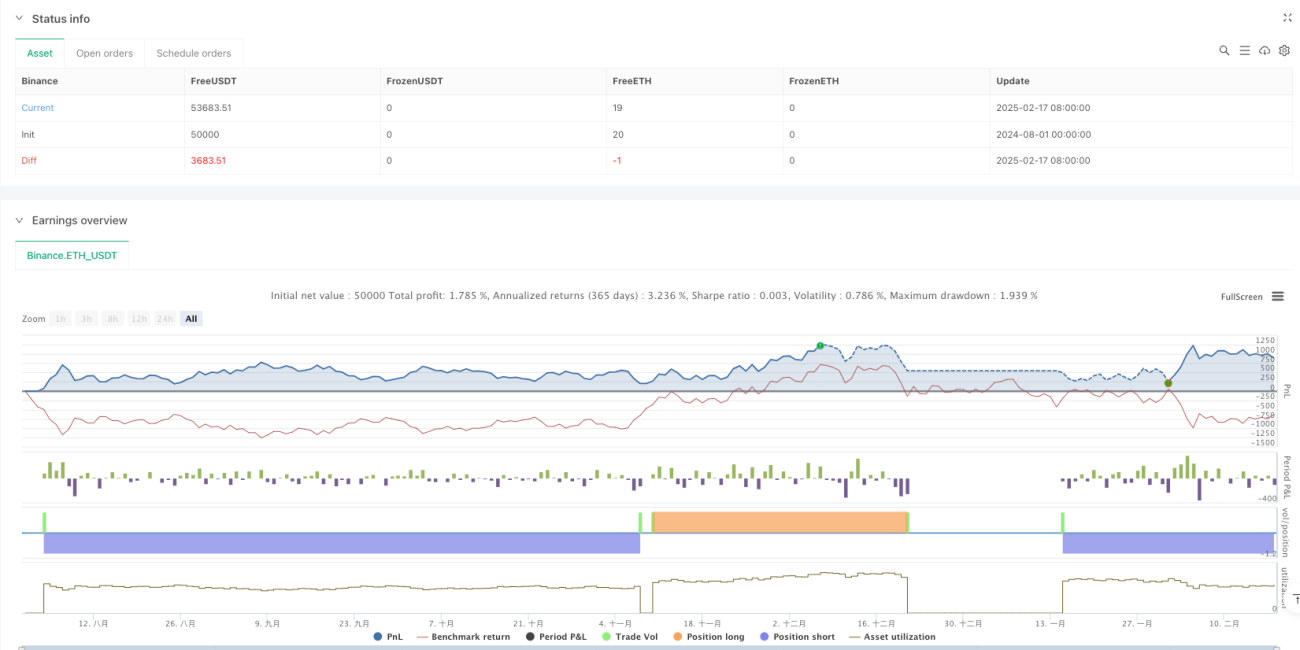
  5. 높은 시간 주기의 우수한 성능: 일계 주기에 2.159의 이익 인수, 당기순 이익 10.71%

전략적 위험

  1. 낮은 승률: 각 시간 주기에서 40% 이하의 승률, 강한 심리적 인내력이 필요합니다.
  2. 낮은 시간 주기의 과도한 거래: 4 시간 주기에 430 개의 거래가 수행되었으며 효율성이 낮습니다.
  3. 신호 지연: 다중 지표 검증을 사용하여 시장 기회를 놓칠 수 있습니다.
  4. 매개 변수 최적화: 여러 지표의 조합은 전략 최적화의 복잡성을 증가시킵니다.

전략 최적화 방향

  1. 신호 필터링 최적화: 각 지표의 마이너스를 조정하여 승률을 높일 수 있습니다.
  2. 시간주기 적응: 주로 일선 및 그 이상의 주기에 사용하는 것이 권장되며, 다른 시장 특성에 따라 매개 변수를 조정할 수 있습니다.
  3. 스톱로스 최적화: 다양한 시장 상황에 따라 ATR 배수를 조정하는 것을 고려할 수 있습니다.
  4. 진입 시간 최적화: 진입 정확성을 높이기 위해 수량 확인 또는 가격 형식 확인을 추가할 수 있습니다.
  5. 포지션 관리 최적화: 신호 강도에 따라 동적 포지션 관리 시스템을 설계할 수 있다

요약하다

이 전략은 합리적이고 논리적으로 명확하게 설계된 통합 거래 시스템으로, 여러 지표의 조합 사용으로 시장 상태를 지능적으로 식별하고 거래 기회를 정확하게 포착합니다. 낮은 시간 주기에는 몇 가지 문제가 있지만, 일선과 같은 높은 시간 주기에는 우수한 성능을 나타냅니다. 거래자는 실장에서 사용할 때 일선 수준의 신호에 중점을 두어 자신의 위험 감수 능력에 따라 합리적으로 매개 변수를 조정하는 것이 좋습니다. 지속적인 최적화 및 조정으로 이 전략은 거래 제공자에게 안정적인 수익 기회를 제공 할 것으로 기대됩니다.

전략 소스 코드
/*backtest
start: 2024-08-01 00:00:00
end: 2025-02-18 08:00:00
period: 2d
basePeriod: 2d
exchanges: [{"eid":"Binance","currency":"ETH_USDT"}]
*/

// This Pine Script™ code is subject to the terms of the Mozilla Public License 2.0 at https://mozilla.org/MPL/2.0/
// © FIWB

//@version=6
strategy("Refined Ichimoku with MACD and RSI Strategy", overlay=true)

// Inputs for Ichimoku Cloud
conversionLength = input.int(9, title="Conversion Line Length", group="Ichimoku Settings")
baseLength = input.int(26, title="Base Line Length", group="Ichimoku Settings")
laggingSpanLength = input.int(52, title="Lagging Span Length", group="Ichimoku Settings")
displacement = input.int(26, title="Displacement", group="Ichimoku Settings")

// Inputs for MACD
macdFastLength = input.int(12, title="MACD Fast Length", group="MACD Settings")
macdSlowLength = input.int(26, title="MACD Slow Length", group="MACD Settings")
macdSignalLength = input.int(9, title="MACD Signal Length", group="MACD Settings")

// Inputs for RSI/Stochastic RSI
rsiLength = input.int(14, title="RSI Length", group="Momentum Indicators")
stochRsiLength = input.int(14, title="Stochastic RSI Length", group="Momentum Indicators")
stochRsiK = input.int(3, title="%K Smoothing", group="Momentum Indicators")
stochRsiD = input.int(3, title="%D Smoothing", group="Momentum Indicators")

// Inputs for ATR
atrLength = input.int(14, title="ATR Length", group="Risk Management")
atrMultiplier = input.float(2.0, title="ATR Multiplier", group="Risk Management")

// Ichimoku Cloud Calculation
conversionLine = (ta.highest(high, conversionLength) + ta.lowest(low, conversionLength)) / 2
baseLine = (ta.highest(high, baseLength) + ta.lowest(low, baseLength)) / 2
leadingSpanA = (conversionLine + baseLine) / 2
leadingSpanB = (ta.highest(high, laggingSpanLength) + ta.lowest(low, laggingSpanLength)) / 2

// Market Regime Detection Using Ichimoku Cloud
priceAboveCloud = close >= leadingSpanA and close >= leadingSpanB
priceBelowCloud = close <= leadingSpanA and close <= leadingSpanB
priceNearCloud = close > leadingSpanB and close < leadingSpanA

trendingMarket = priceAboveCloud or priceBelowCloud
rangeBoundMarket = priceNearCloud

// MACD Calculation
macdLine = ta.ema(close, macdFastLength) - ta.ema(close, macdSlowLength)
macdSignalLine = ta.sma(macdLine, macdSignalLength)
macdHistogram = macdLine - macdSignalLine

// RSI Calculation
rsiValue = ta.rsi(close, rsiLength)

// Stochastic RSI Calculation
stochRsiKValue = ta.sma(ta.stoch(close, high, low, stochRsiLength), stochRsiK)
stochRsiDValue = ta.sma(stochRsiKValue, stochRsiD)

// Entry Conditions with Tightened Filters
trendLongCondition = trendingMarket and priceAboveCloud and rsiValue > 55 and macdHistogram > 0 and stochRsiKValue > stochRsiDValue
trendShortCondition = trendingMarket and priceBelowCloud and rsiValue < 45 and macdHistogram < 0 and stochRsiKValue < stochRsiDValue

rangeLongCondition = rangeBoundMarket and rsiValue < 30 and stochRsiKValue < 20
rangeShortCondition = rangeBoundMarket and rsiValue > 70 and stochRsiKValue > 80

// Risk Management: Stop-Loss Based on ATR
atrValue = ta.atr(atrLength)
longStopLoss = low - atrMultiplier * atrValue
shortStopLoss = high + atrMultiplier * atrValue

// Strategy Execution: Entries and Exits
if trendLongCondition
    strategy.entry("Trend Long", strategy.long)
    strategy.exit("Exit Trend Long", from_entry="Trend Long", stop=longStopLoss)

if trendShortCondition
    strategy.entry("Trend Short", strategy.short)
    strategy.exit("Exit Trend Short", from_entry="Trend Short", stop=shortStopLoss)

if rangeLongCondition
    strategy.entry("Range Long", strategy.long)
    strategy.exit("Exit Range Long", from_entry="Range Long", stop=longStopLoss)

if rangeShortCondition
    strategy.entry("Range Short", strategy.short)
    strategy.exit("Exit Range Short", from_entry="Range Short", stop=shortStopLoss)

// Visualization: Highlight Market Regimes on Chart Background
bgcolor(trendingMarket ? color.new(color.green, 90) : na)
bgcolor(rangeBoundMarket ? color.new(color.red, 90) : na)

// Plot Ichimoku Cloud for Visualization
plot(leadingSpanA, color=color.new(color.green, 80), title="Leading Span A")
plot(leadingSpanB, color=color.new(color.red, 80), title="Leading Span B")