나다라야-왓슨 기반의 다차원 통합 거래 전략

2
Follow
478
Followers

개요
이 전략은 Nadaraya-Watson 핵 회귀를 기반으로 한 다차원 거래 시스템으로, 기술, 감정, 초감각 및 의지의 4 차원의 시장 정보를 통합하여 통합된 신호를 형성하여 거래 결정을 안내합니다. 전략은 무게 최적화 방법을 채택하여 다양한 차원의 신호를 가중 처리하고, 신호 품질을 높이기 위해 추세와 동력 필터를 결합합니다.
전략 원칙
전략의 핵심은 Nadaraya-Watson 핵 회귀 방법을 통해 여러 차원의 시장 데이터를 부드럽게 처리하는 것입니다. 구체적으로:
- 기술 차원 사용 종식 가격
- 감정 차원은 RSI 지표를 사용한다.
- 초감각 차원 사용 ATR 변동률
- 의도적인 차원 사용 가격과 평균 선의 편차
이 차원은 핵 회귀를 평형화 한 후, 전설 중량 ((기술 0.4, 감정 0.2, 초감정 0.2, 의향 0.2) 을 통해 중량 통합을 통해 최종 거래 신호를 형성한다. 통합 신호가 이동 평균과 교차 할 때, 추세와 운동량 필터 확인 후 거래 지시가 발령된다.
전략적 이점
- 다차원 분석은 단일 지표의 한계를 피하여 더 포괄적인 시장 관점을 제공합니다.
- 나다라야-왓슨 핵 회귀는 시장의 소음을 효과적으로 줄여서 더 부드러운 신호를 제공합니다.
- 무게 최적화 메커니즘은 시장 특성에 따라 각 차원의 중요성을 조정할 수 있습니다.
- 트렌드 및 동력 필터의 추가로 신호 품질이 크게 향상되었습니다.
- 좋은 리스크 관리 시스템으로 자금의 안전성을 보장합니다.
전략적 위험
- 과도한 매개변수 최적화는 과적합으로 이어질 수 있습니다.
- 복수의 필터링 조건이 유효한 신호의 일부를 놓칠 수 있습니다.
- 핵 회귀 계산의 복잡성이 높으며, 실시간 성능에 영향을 미칠 수 있다.
- 부적절한 무게분배는 중요한 시장 신호를 약화시킬 수 있습니다.
완화 조치에는: 샘플 외 테스트 검증 파라미터를 사용, 필터링 조건을 동적으로 조정, 계산 효율을 최적화, 주기적으로 평가 및 무게 분배를 조정하는 등이 포함됩니다.
전략 최적화 방향
- 시장 상황에 따라 각 차원의 무게를 조정하는 적응형 무게 시스템을 도입합니다.
- 더 지능적인 필터링 메커니즘을 개발하여 신호의 양과 질을 균형을 잡습니다.
- 나다라야-왓슨 알고리즘 구현을 최적화하여 계산 효율을 높인다.
- 시장 주기를 인식하는 모듈을 추가하여 다른 시장 단계에서 다른 파라미터 설정을 사용합니다.
- 위험 관리 시스템을 확장하고, 동적 중지 및 포지션 관리 기능을 추가
요약하다
이것은 수학적 방법과 거래의 지능을 결합하는 혁신적인 전략이다. 다차원 분석과 첨단 수학적 도구를 통해 전략은 시장의 여러 층을 포착하여 상대적으로 신뢰할 수있는 거래 신호를 제공합니다. 일부 최적화 공간이 있지만 전략의 전체적인 프레임 워크는 견고하고 실제 응용 가치가 있습니다.
Source
Pine
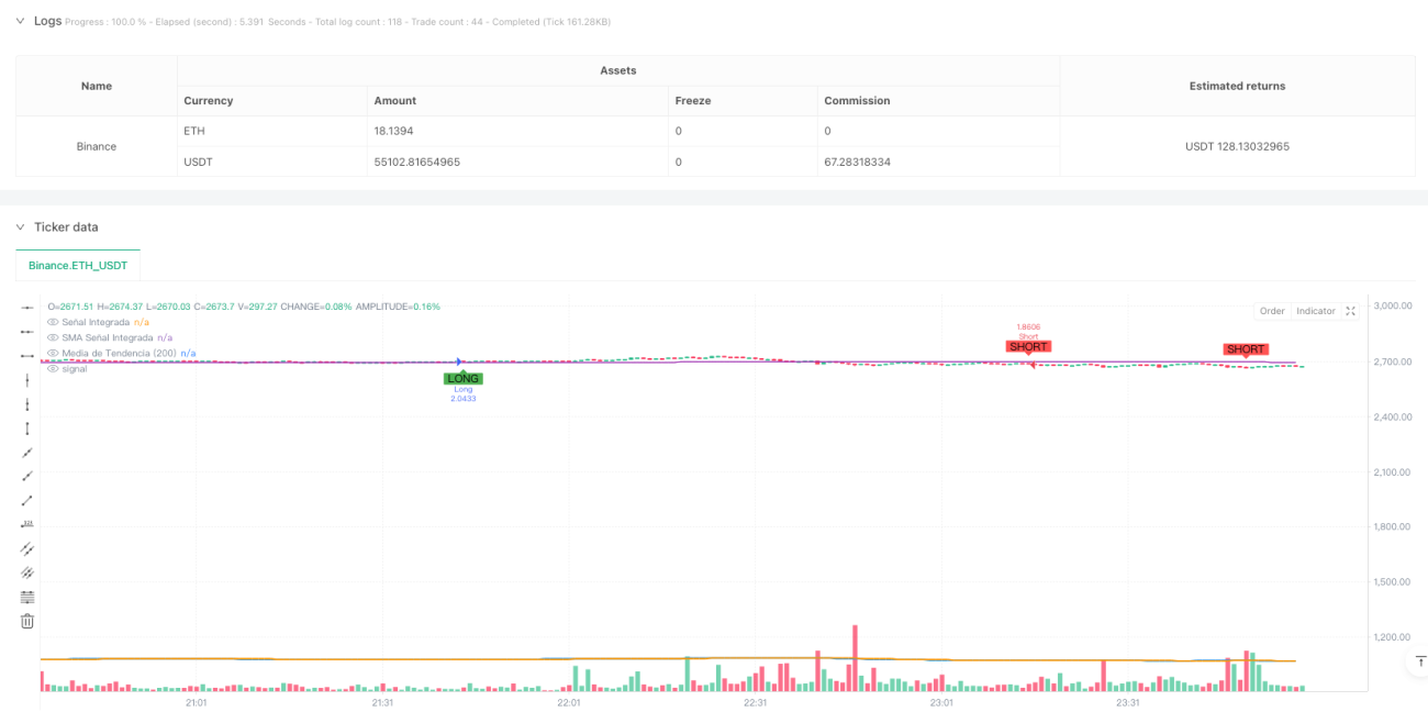
/*backtest
start: 2025-02-17 00:00:00
end: 2025-02-19 00:00:00
period: 1m
basePeriod: 1m
exchanges: [{"eid":"Binance","currency":"ETH_USDT"}]
*/

//@version=5
strategy("Enhanced Multidimensional Integration Strategy with Nadaraya", overlay=true, initial_capital=10000, currency=currency.USD, default_qty_type=strategy.percent_of_equity, default_qty_value=10)

//────────────────────────────────────────────────────────────────────────────Strategy parameters
Related strategies
Comment
All comments (0)
No data
- 1