
다중 지표 트렌드 라인 크로스 동적 중지 손실 수량 거래 전략은 트렌드 라인 분석, 기술 지표 및 위험 관리를 결합 한 통합 거래 시스템입니다. 이 전략의 핵심은 선형 회귀법을 통해 동적 트렌드 라인을 구성하고 RSI, MACD, 거래량 및 시장 구조 분석을 결합하여 높은 확률의 거래 기회를 식별합니다. 이 전략은 ATR 동적 중지 손실을 사용하여 위험 비율 방식을 사용하여 포지션 관리를 수행하고 이중 수익 목표를 설정합니다. 이 전략은 특히 변동성이 높은 시장에 적합하며, 여러 확인 장치와 엄격한 위험 제어로 거래 성공률을 높입니다.
이 전략은 다음과 같은 핵심 원칙에 기초하고 있습니다.
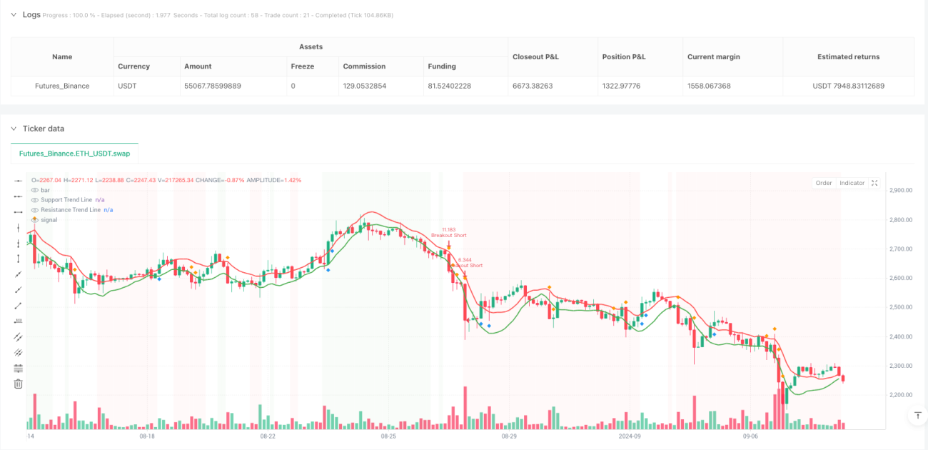
동적 트렌드 라인 식별: 선형 회귀 (Linear Regression) 기술을 사용하여 지지 및 저항 트렌드 라인을 구성하고, 가격과 트렌드 라인의 관계를 분석하여 잠재적인 반발 및 거부점을 식별한다.
다중 지표 공명 확인:
트레이딩 메커니즘을 뚫고: 거래량과 함께 가격이 저항 또는 지지를 돌파하면 거래 신호를 니다.
위험 관리 시스템:
트랜잭션 실행 논리:
전체적인 시장 분석: 트렌드 라인, 쇼크 지표, 동력 지표 및 거래량 분석을 포함한 여러 기술 분석 방법을 결합하여 더 포괄적인 시장 관점을 제공하여 잘못된 신호를 줄입니다.
동적으로 시장 조건에 적응: 트렌드 라인은 선형 회귀를 통해 동적으로 계산되며, 상이한 시장 환경에 적응할 수 있으며, 정적 지지 저항 지점보다 더 유연하다.
다중 인증 메커니즘: 여러 조건이 동시에 충족되어야 거래 신호가 발생하여 신호 품질이 크게 향상되고 잘못된 거래가 감소합니다.
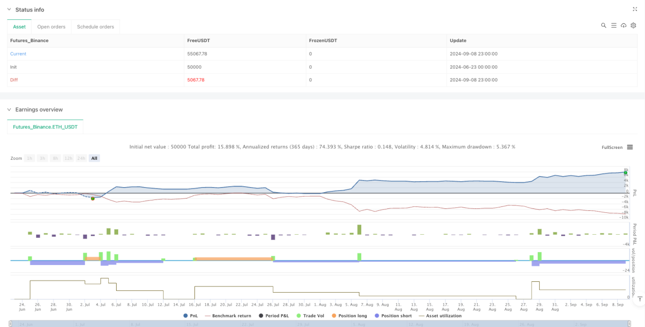
좋은 위험 관리:
시각적 피드백전략은 트렌드 라인, 신호 및 시장 상태에 대한 시각적 피드백을 제공하여 거래자가 시장 환경과 전략 수행을 더 잘 이해할 수 있도록 도와줍니다.
유연한 변수 설정: 전략은 사용자가 거래 종류와 개인 위험 선호에 따라 여러 가지 변수를 조정할 수 있도록 허용하여 적응력을 강화합니다.
매개변수 민감도: 전략은 트렌드 라인 길이, RSI 마이너스, MACD 파라미터 등과 같은 여러 파라미터 설정에 의존한다. 부적절한 파라미터 설정은 과도한 거래 또는 놓친 기회를 초래할 수 있다. 해결책은 최적화 파라미터를 재측정하고 다른 시장 조건에 대해 다른 파라미터 설정을 하는 것이다.
다중 조건 거래 빈도 제한다중 확인 메커니즘은 신호 품질을 향상시키지만 거래 기회를 감소시킬 수 있으며, 특정 시장 환경에서 오랫동안 신호를 유발할 수 없습니다. 해결책은 조건 중량 시스템을 추가하여 특정 조건이 특히 강할 때 다른 조건 요구 사항을 완화시키는 것을 고려하는 것입니다.
트렌드 라인 계산의 복잡성: 선형 회귀 트렌드 라인은 일부 극단적 인 시장 조건에서 정확하지 않을 수 있습니다. 특히 급격히 변동하거나 갑자기 변하는 시장에서. 해결책은 다른 지원 저항 식별 방법과 결합하여 결정적 가격 또는 이동 평균과 같은 것입니다.
포지션 계산은 스톱로스에 의존한다전략의 포지션 크기는 스톱포인트 위치에 의존한다. ATR 계산의 스톱포인트 거리가 너무 크면 포지션이 너무 작아 수익 잠재력에 영향을 줄 수 있다. 해결책은 최대 스톱포인트 거리의 제한을 설정하거나 혼합 포지션 계산 방법을 고려하는 것이다.
탈퇴 위험: 위험 관리 장치가 있음에도 불구하고, 급격한 시장 조건에서, 예를 들어, 붕괴 또는 가격 폭파와 같은 경우, 실제 손실이 예상보다 클 수 있습니다.
기계 학습 강화: 기계 학습 알고리즘을 도입하여 자동으로 최적화 변수를 도입하여 다양한 시장 환경의 동성에 따라 RSI 마이너스, MACD 변수 및 트렌드 라인 길이를 조정합니다. 이것은 다양한 시장 단계에서 고정 변수의 한계를 극복하고 전략의 적응성을 향상시킬 수 있습니다.
시장 환경 분류: 시장 환경을 식별하는 시스템을 구현하고, 시장을 트렌드형, 간격형, 전환형 세 가지 상태로 나누고, 각 상태에 대해 다른 거래 규칙을 사용합니다. 이렇게하면 부적절한 시장 환경에서 과도한 거래를 피할 수 있습니다.
지표중력 시스템: 동적 지표 중량 시스템을 구축하여 특정 지표 신호가 특히 강할 때 다른 지표의 중요성을 줄일 수 있습니다. 이것은 여러 확인 우위를 유지하면서 거래 빈도를 증가시킬 수 있습니다.
트렌드 라인 알고리즘 개선: 더 복잡한 트렌드 라인 식별 알고리즘의 사용, 예를 들어 다항적 회귀 또는 지원 벡터 기계 ((SVM), 다양한 시장 조건에서 트렌드 라인의 정확성을 향상.
위험 관리 강화:
감정 지표 통합시장 감정 지표, 예를 들어 변동률 지수 ((VIX) 또는 자본 흐름 데이터를 추가 필터링 조건으로 도입하여 극심한 시장 감정 아래 거래하는 것을 피하십시오.
다중 지표 트렌드 라인 크로스 동적 정지 손실 수량 거래 전략은 트렌드 라인 분석, 기술 지표 및 엄격한 위험 관리를 결합하여 거래자에게 고품질의 거래 신호를 제공하도록 설계된 포괄적 인 거래 시스템입니다. 이 전략의 가장 큰 장점은 다중 확인 장치와 완벽한 위험 제어 시스템입니다. 그러나 파라미터 민감성 및 거래 빈도 제한과 같은 잠재적인 문제에 대해서도 주의해야합니다.
트렌드 라인 알고리즘을 최적화하고, 동적 파라미터 조정을 구현하고, 시장 환경 분류를 도입하고, 리스크 관리 시스템을 강화함으로써, 이 전략은 더욱 안정성과 적응성을 향상시킬 수 있다.
이 전략은 가격 형태, 지표 공명 및 거래량 확인을 포함한 기술 분석의 여러 차원을 결합하여 통합 된 거래 의사 결정 시스템을 형성합니다. 엄격한 입시 조건과 명확한 위험 관리 규칙으로 인해 훈련 된 거래 방법을 제공하여 거래자가 변동하는 시장에서 정서적 안정성을 유지하고 일관된 거래 계획을 수행 할 수 있습니다.
/*backtest
start: 2024-06-23 00:00:00
end: 2024-09-09 00:00:00
period: 3h
basePeriod: 3h
exchanges: [{"eid":"Futures_Binance","currency":"ETH_USDT"}]
*/
//@version=5
strategy("Advanced Crypto Trend Line Strategy", overlay=true, margin_long=100, margin_short=100)
// ================================
// INPUT PARAMETERS
// ================================
// Crypto Selection
crypto_type = input.string("BTC", "Cryptocurrency", options=["BTC", "SOL", "AUTO"])
// Trend Line Parameters
trendline_length = input.int(20, "Trend Line Calculation Length", minval=10, maxval=50)
min_touches = input.int(2, "Minimum Trend Line Touches", minval=2, maxval=5)
breakout_threshold = input.float(0.5, "Breakout Threshold %", minval=0.1, maxval=2.0) / 100
// Risk Management
risk_percent = input.float(2.0, "Risk Per Trade %", minval=0.5, maxval=5.0) / 100
tp1_ratio = input.float(2.0, "Take Profit 1 Ratio", minval=1.0, maxval=5.0)
tp2_ratio = input.float(3.0, "Take Profit 2 Ratio", minval=2.0, maxval=6.0)
max_leverage = crypto_type == "BTC" ? 5 : crypto_type == "SOL" ? 10 : 7
// Technical Indicators
rsi_length = input.int(14, "RSI Length", minval=5, maxval=30)
rsi_oversold = input.int(35, "RSI Oversold Level", minval=20, maxval=40)
rsi_overbought = input.int(70, "RSI Overbought Level", minval=60, maxval=80)
macd_fast = input.int(12, "MACD Fast Length", minval=5, maxval=20)
macd_slow = input.int(26, "MACD Slow Length", minval=20, maxval=40)
macd_signal = input.int(9, "MACD Signal Length", minval=5, maxval=15)
volume_multiplier = input.float(1.5, "Volume Spike Multiplier", minval=1.1, maxval=3.0)
// ATR for Dynamic Stops
atr_length = input.int(14, "ATR Length for Stops", minval=5, maxval=30)
atr_multiplier = input.float(2.0, "ATR Stop Multiplier", minval=1.0, maxval=4.0)
// ================================
// TECHNICAL INDICATORS
// ================================
// RSI
rsi = ta.rsi(close, rsi_length)
// MACD
[macd_line, signal_line, macd_histogram] = ta.macd(close, macd_fast, macd_slow, macd_signal)
// Volume
volume_avg = ta.sma(volume, 20)
volume_spike = volume > volume_avg * volume_multiplier
// ATR for dynamic stops
atr = ta.atr(atr_length)
// ================================
// TREND LINE CALCULATION
// ================================
// Function to calculate trend line slope and intercept
get_trend_line(src, len, min_touch) =>
var float slope = na
var float intercept = na
var int touches = 0
var array<float> highs = array.new<float>()
var array<float> lows = array.new<float>()
var array<int> high_bars = array.new<int>()
var array<int> low_bars = array.new<int>()
// Find pivots
ph = ta.pivothigh(high, 5, 5)
pl = ta.pivotlow(low, 5, 5)
// Store pivot points
if not na(ph)
array.push(highs, ph)
array.push(high_bars, bar_index - 5)
if array.size(highs) > len
array.shift(highs)
array.shift(high_bars)
if not na(pl)
array.push(lows, pl)
array.push(low_bars, bar_index - 5)
if array.size(lows) > len
array.shift(lows)
array.shift(low_bars)
[slope, intercept, touches]
// Calculate trend lines
[up_slope, up_intercept, up_touches] = get_trend_line(low, trendline_length, min_touches)
[down_slope, down_intercept, down_touches] = get_trend_line(high, trendline_length, min_touches)
// ================================
// TREND LINE VALUES
// ================================
// Simplified trend line calculation using linear regression
uptrend_line = ta.linreg(low, trendline_length, 0)
downtrend_line = ta.linreg(high, trendline_length, 0)
// Dynamic trend line based on recent pivots
recent_low = ta.lowest(low, 10)
recent_high = ta.highest(high, 10)
// Support and Resistance levels
support_level = uptrend_line
resistance_level = downtrend_line
// ================================
// MARKET STRUCTURE
// ================================
// Higher lows and lower highs detection
higher_low = low > ta.lowest(low[1], 5) and low[1] > ta.lowest(low[2], 5)
lower_high = high < ta.highest(high[1], 5) and high[1] < ta.highest(high[2], 5)
// Overall trend determination
uptrend = close > ta.sma(close, 50) and ta.sma(close, 20) > ta.sma(close, 50)
downtrend = close < ta.sma(close, 50) and ta.sma(close, 20) < ta.sma(close, 50)
// ================================
// ENTRY CONDITIONS
// ================================
// Long entry conditions
long_trend_bounce = close > support_level and low <= support_level * 1.01
long_rsi = rsi < rsi_oversold or (rsi > rsi_oversold and rsi[1] < rsi_oversold)
long_macd = macd_histogram > macd_histogram[1]
long_volume = volume_spike
long_structure = higher_low or uptrend
long_condition = long_trend_bounce and long_rsi and long_macd and long_volume and long_structure
// Short entry conditions
short_trend_reject = close < resistance_level and high >= resistance_level * 0.99
short_rsi = rsi > rsi_overbought or (rsi < rsi_overbought and rsi[1] > rsi_overbought)
short_macd = macd_histogram < macd_histogram[1]
short_volume = volume_spike
short_structure = lower_high or downtrend
short_condition = short_trend_reject and short_rsi and short_macd and short_volume and short_structure
// ================================
// BREAKOUT CONDITIONS
// ================================
// Uptrend breakout (bearish)
uptrend_break = close < support_level * (1 - breakout_threshold) and volume_spike
// Downtrend breakout (bullish)
downtrend_break = close > resistance_level * (1 + breakout_threshold) and volume_spike
// ================================
// POSITION SIZING
// ================================
// Calculate position size based on risk
account_size = strategy.equity
risk_amount = account_size * risk_percent
// ================================
// STRATEGY EXECUTION
// ================================
// Long entries
if long_condition and strategy.position_size == 0
stop_loss = support_level - (atr * atr_multiplier)
take_profit_1 = close + (close - stop_loss) * tp1_ratio
take_profit_2 = close + (close - stop_loss) * tp2_ratio
// Position sizing
risk_per_share = close - stop_loss
position_size = risk_amount / risk_per_share
position_size := math.min(position_size, account_size * max_leverage / close)
strategy.entry("Long", strategy.long, qty=position_size)
strategy.exit("Long TP1", "Long", limit=take_profit_1, stop=stop_loss, qty=position_size * 0.5)
strategy.exit("Long TP2", "Long", limit=take_profit_2, stop=stop_loss, qty=position_size * 0.5)
// Short entries
if short_condition and strategy.position_size == 0
stop_loss = resistance_level + (atr * atr_multiplier)
take_profit_1 = close - (stop_loss - close) * tp1_ratio
take_profit_2 = close - (stop_loss - close) * tp2_ratio
// Position sizing
risk_per_share = stop_loss - close
position_size = risk_amount / risk_per_share
position_size := math.min(position_size, account_size * max_leverage / close)
strategy.entry("Short", strategy.short, qty=position_size)
strategy.exit("Short TP1", "Short", limit=take_profit_1, stop=stop_loss, qty=position_size * 0.5)
strategy.exit("Short TP2", "Short", limit=take_profit_2, stop=stop_loss, qty=position_size * 0.5)
// Breakout entries
if downtrend_break and strategy.position_size == 0
stop_loss = resistance_level - (atr * atr_multiplier)
take_profit = close + (close - stop_loss) * 2.0
risk_per_share = close - stop_loss
position_size = risk_amount / risk_per_share
position_size := math.min(position_size, account_size * max_leverage / close)
strategy.entry("Breakout Long", strategy.long, qty=position_size)
strategy.exit("Breakout Long Exit", "Breakout Long", limit=take_profit, stop=stop_loss)
if uptrend_break and strategy.position_size == 0
stop_loss = support_level + (atr * atr_multiplier)
take_profit = close - (stop_loss - close) * 2.0
risk_per_share = stop_loss - close
position_size = risk_amount / risk_per_share
position_size := math.min(position_size, account_size * max_leverage / close)
strategy.entry("Breakout Short", strategy.short, qty=position_size)
strategy.exit("Breakout Short Exit", "Breakout Short", limit=take_profit, stop=stop_loss)
// ================================
// VISUALIZATION
// ================================
// Plot trend lines
plot(support_level, "Support Trend Line", color=color.green, linewidth=2)
plot(resistance_level, "Resistance Trend Line", color=color.red, linewidth=2)
// Plot entry signals
plotshape(long_condition, "Long Signal", shape.triangleup, location.belowbar, color.green, size=size.small)
plotshape(short_condition, "Short Signal", shape.triangledown, location.abovebar, color.red, size=size.small)
// Plot breakout signals
plotshape(downtrend_break, "Bullish Breakout", shape.diamond, location.belowbar, color.blue, size=size.small)
plotshape(uptrend_break, "Bearish Breakout", shape.diamond, location.abovebar, color.orange, size=size.small)
// Background color for trend
bgcolor(uptrend ? color.new(color.green, 95) : downtrend ? color.new(color.red, 95) : na)
// ================================
// ALERTS
// ================================
// Entry alerts
alertcondition(long_condition, "Long Entry", "Long entry signal detected")
alertcondition(short_condition, "Short Entry", "Short entry signal detected")
alertcondition(downtrend_break, "Bullish Breakout", "Bullish breakout detected")
alertcondition(uptrend_break, "Bearish Breakout", "Bearish breakout detected")
// ================================
// TABLE FOR INFORMATION
// ================================
// Create info table
var table info_table = table.new(position.top_right, 2, 8, bgcolor=color.white, border_width=1)
if barstate.islast
table.cell(info_table, 0, 0, "Metric", text_color=color.black, bgcolor=color.gray)
table.cell(info_table, 1, 0, "Value", text_color=color.black, bgcolor=color.gray)
table.cell(info_table, 0, 1, "RSI", text_color=color.black)
table.cell(info_table, 1, 1, str.tostring(math.round(rsi, 2)), text_color=color.black)
table.cell(info_table, 0, 2, "MACD", text_color=color.black)
table.cell(info_table, 1, 2, str.tostring(math.round(macd_line, 4)), text_color=color.black)
table.cell(info_table, 0, 3, "Volume Spike", text_color=color.black)
table.cell(info_table, 1, 3, volume_spike ? "YES" : "NO", text_color=color.black)
table.cell(info_table, 0, 4, "Trend", text_color=color.black)
table.cell(info_table, 1, 4, uptrend ? "UP" : downtrend ? "DOWN" : "SIDEWAYS", text_color=color.black)
table.cell(info_table, 0, 5, "Support", text_color=color.black)
table.cell(info_table, 1, 5, str.tostring(math.round(support_level, 2)), text_color=color.black)
table.cell(info_table, 0, 6, "Resistance", text_color=color.black)
table.cell(info_table, 1, 6, str.tostring(math.round(resistance_level, 2)), text_color=color.black)
table.cell(info_table, 0, 7, "ATR", text_color=color.black)
table.cell(info_table, 1, 7, str.tostring(math.round(atr, 2)), text_color=color.black)