K-algo 추세 추종 전략

ATR supertrend GANN HEIKIN-ASHI EMA
생성 날짜: 2025-08-26 11:23:33 마지막으로 수정됨: 2025-08-26 11:23:33
복사: 0 클릭수: 288
avatar of ianzeng123 ianzeng123
2
집중하다
319
수행원

K-algo 추세 추종 전략 K-algo 추세 추종 전략

이것은 일반적인 슈퍼트렌드가 아니라, 다차원적 융합의 트렌드 사냥꾼입니다.

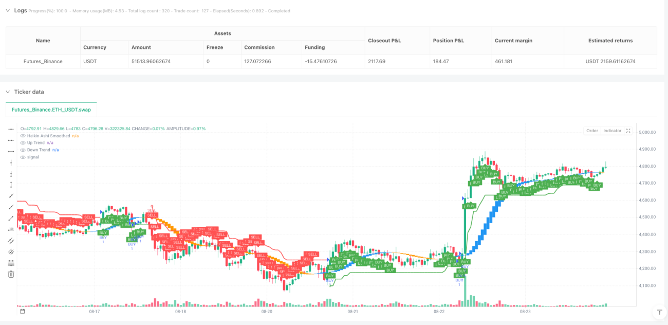
이름에 속지 마세요, K-algo trail은 단순한 ATR 추적 전략이 아닙니다. 이 시스템은 SuperTrend, Gann 9 차원 그래프, Heikin Ashi의 세 가지 기술 체계를 교묘하게 결합하여 3 차원 트렌드 식별 프레임 워크를 형성합니다. 10 주기 ATR은 3 배수의 배수와 함께 설계되어 트렌드에 대한 민감성을 보장하고 시장 소음을 효과적으로 필터링합니다.

이중 EMA 부드러운 Heikin Ashi가 진정한 신호 필터입니다.

전략의 핵심 혁신은 쌍 11주기 EMA 평준화 처리된 Heikin Ashi 도표에 있다. 전통적인 Heikin Ashi는 가짜 신호를 발생시키는데, 2회 EMA 평준화 이후에는 신호 품질이 눈에 띄게 향상된다. 평준화 후의 개시 가격이 종점 가격보다 낮아지고 SuperTrend이 상승세를 보였을 때, 다단계 신호가 확인된다. 반대로 공백 신호이다. 이 쌍 확인 메커니즘은 잘못된 거래의 가능성을 크게 감소시킨다.

1.7:2.5:3.0의 수익과 손실은 디자인에 대한 전문성을 나타냅니다.

손해 중지 설정은 SuperTrend 선 지점을 직접 적용하는 것이 가장 합리적인 다이내믹 스톱 옵션입니다. 더 흥미로운 것은 세 단계의 스톱 디자인이 있습니다: 1.7 배, 2.5 배, 3.0 배의 위험 거리입니다. 이러한 점진적인 스톱은 기본 수익을 보장하고 트렌드 상황에 충분한 공간을 남깁니다. 역사적으로 이러한 비율은 대부분의 시장 환경에서 기대되는 수익을 달성 할 수 있습니다.

Gann의 9자 도표가 추가된 것은 장식품이 아니라, 저항을 지지하는 핵심 요소입니다.

코드에 있는 Gann Square of 9 계산은 단순해 보이지만 실제적으로 큰 역할을 한다. 현재 가격의 제곱근을 계산하여 위아래의 지지 저항 지점을 계산하여 전략에 대해 추가적인 가격 포인트를 제공한다. 전략주석 논리가 직접적으로 이러한 위치를 사용하지 않음에도 불구하고, 그것들은 수동 조정 및 위험 평가에 대한 중요한 참조를 제공한다.

중·장기 추세 상황, 변동성 시장의 일반적인 성과에 적용됩니다.

이 전략은 일방적인 트렌드 시장에서 우수한 성능을 발휘합니다. 특히 암호화폐와 주식 지수 선물과 같은 변동성이 높은 품종이 있습니다. 그러나 명확하게해야합니다. 수평 변동 상황에서 빈번한 가짜 돌파는 연속으로 작은 손실을 초래합니다. 시장의 변동성이 높고 트렌드성이 강한 시기에 사용하는 것이 좋습니다. 중요한 경제 데이터가 발표되기 전의 불확실한 기간을 피하십시오.

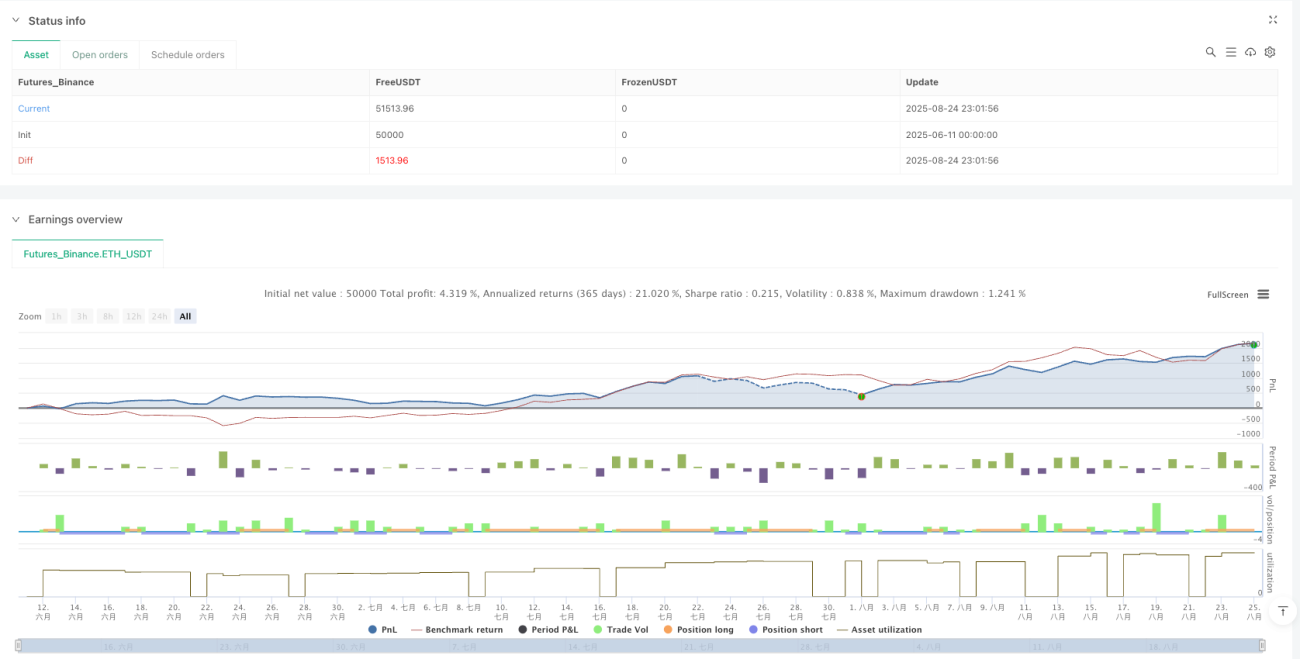
리스크 팁: 과거 회귀는 미래 수익을 의미하지 않습니다.

모든 양적 전략에는 손실의 위험이 존재하며, 이 전략도 예외는 아니다. 재검토 데이터는 위험 조정 후 수익이 좋은 것으로 나타났지만, 실제 거래에서는 연속적인 손실이 발생할 수 있다. 단일 포지션은 총 자본의 2%를 초과하지 않도록 엄격하게 통제하고, 연속적으로 3 번의 손실이 발생한 후 거래를 중단하고 시장 환경을 재평가하는 것이 좋습니다. 전략의 효과는 시장 추세에 크게 의존하며, 명확한 방향이없는 시장에서 신중하게 사용해야합니다.

전략 소스 코드
/*backtest
start: 2025-06-11 00:00:00
end: 2025-08-25 00:00:00
period: 1h
basePeriod: 1h
exchanges: [{"eid":"Futures_Binance","currency":"ETH_USDT"}]
*/

//@version=5
strategy('K-algo trail', overlay=true)
// ===== INPUTS =====
Periods = input(title='ATR Period', defval=10)
src = input(hl2, title='Source')
Multiplier = input.float(title='ATR Multiplier', step=0.1, defval=3)
changeATR = input(title='Change ATR Calculation Method ?', defval=true)
showsignals = input(title='Show Buy/Sell Signals ?', defval=true)
// ===== ATR & SUPER TREND (K-TREND) CALCULATION =====
atr2 = ta.sma(ta.tr, Periods)
atr = changeATR ? ta.atr(Periods) : atr2
up = src - Multiplier * atr
up1 = nz(up[1], up)
up := close[1] > up1 ? math.max(up, up1) : up
dn = src + Multiplier * atr
dn1 = nz(dn[1], dn)
dn := close[1] < dn1 ? math.min(dn, dn1) : dn
trend = 1
trend := nz(trend[1], trend)
trend := trend == -1 and close > dn1 ? 1 : trend == 1 and close < up1 ? -1 : trend
// Plot SuperTrend
upPlot = plot(trend == 1 ? up : na, title='Up Trend', style=plot.style_linebr, linewidth=2, color=color.new(color.green, 0))
buySignal = trend == 1 and trend[1] == -1
plotshape(buySignal ? up : na, title='UpTrend Begins', location=location.absolute, style=shape.circle, size=size.tiny, color=color.new(color.green, 0))
dnPlot = plot(trend == 1 ? na : dn, title='Down Trend', style=plot.style_linebr, linewidth=2, color=color.new(color.red, 0))
sellSignal = trend == -1 and trend[1] == 1
plotshape(sellSignal ? dn : na, title='DownTrend Begins', location=location.absolute, style=shape.circle, size=size.tiny, color=color.new(color.red, 0))
// ===== GANN SQUARE OF 9 =====
normalise_squareRootCurrentClose = math.floor(math.sqrt(close))
upperGannLevel_1 = (normalise_squareRootCurrentClose + 1) * (normalise_squareRootCurrentClose + 1)
upperGannLevel_2 = (normalise_squareRootCurrentClose + 2) * (normalise_squareRootCurrentClose + 2)
zeroGannLevel = normalise_squareRootCurrentClose * normalise_squareRootCurrentClose
lowerGannLevel_1 = (normalise_squareRootCurrentClose - 1) * (normalise_squareRootCurrentClose - 1)
lowerGannLevel_2 = (normalise_squareRootCurrentClose - 2) * (normalise_squareRootCurrentClose - 2)
// ===== SMOOTHED HEIKIN ASHI CALCULATION =====
ma1_len = input.int(title='MA1', defval=11, minval=1, maxval=100, step=1)
ma2_len = input.int(title='MA2', defval=11, minval=1, maxval=100, step=1)
// First Smoothing (11,11)
o = ta.ema(open, ma1_len)
c = ta.ema(close, ma1_len)
h = ta.ema(high, ma1_len)
l = ta.ema(low, ma1_len)
ha_t = ticker.heikinashi(syminfo.tickerid)
ha_o = request.security(ha_t, timeframe.period, o)
ha_c = request.security(ha_t, timeframe.period, c)
ha_h = request.security(ha_t, timeframe.period, h)
ha_l = request.security(ha_t, timeframe.period, l)
o2 = ta.ema(ha_o, ma2_len)
c2 = ta.ema(ha_c, ma2_len)
h2 = ta.ema(ha_h, ma2_len)
l2 = ta.ema(ha_l, ma2_len)
ha_col = o2 > c2 ? color.orange : color.blue
plotcandle(o2, h2, l2, c2, title='Heikin Ashi Smoothed', color=ha_col, wickcolor=#00000000)
// ===== STRATEGY LOGIC =====
// Final Combined Long Condition
longCondition = (o2 < c2 and trend == 1) and barstate.isconfirmed
// Final Combined Short Condition
shortCondition = (o2 > c2 and trend == -1) and barstate.isconfirmed
// ===== STRATEGY EXECUTION =====
if longCondition
    SL = math.round(up, 2)
    range_1 = math.abs(close - SL)
    TARGET1 = close + range_1 * 1.7
    TARGET2 = close + range_1 * 2.5
    TARGET3 = close + range_1 * 3.0
    strategy.entry('BUY', strategy.long)
    strategy.exit('BUY T1', 'BUY', qty=1, limit=TARGET1)
    strategy.exit('BUY T2', 'BUY', qty=1, limit=TARGET2)
    strategy.exit('BUY T3', 'BUY', qty=1, limit=TARGET3)
    strategy.exit('BUY SL', 'BUY', stop=SL)
if shortCondition
    SL = math.round(dn, 2)
    range_2 = math.abs(close - SL)
    TARGET1 = close - range_2 * 1.7
    TARGET2 = close - range_2 * 2.5
    TARGET3 = close - range_2 * 3.0
    strategy.entry('SELL', strategy.short)
    strategy.exit('SELL T1', 'SELL', qty=1, limit=TARGET1)
    strategy.exit('SELL T2', 'SELL', qty=1, limit=TARGET2)
    strategy.exit('SELL T3', 'SELL', qty=1, limit=TARGET3)
    strategy.exit('SELL SL', 'SELL', stop=SL)
// Plot entry signals
plotshape(longCondition ? close : na, title='Buy', text='BUY', location=location.belowbar, style=shape.labelup, size=size.tiny, color=color.new(color.green, 0), textcolor=color.new(color.white, 0))
plotshape(shortCondition ? close : na, title='Sell', text='SELL', location=location.abovebar, style=shape.labeldown, size=size.tiny, color=color.new(color.red, 0), textcolor=color.new(color.white, 0))