Strategi perdagangan momentum pelbagai dimensi berdasarkan analisis spektrum kuantum

Gambaran keseluruhan
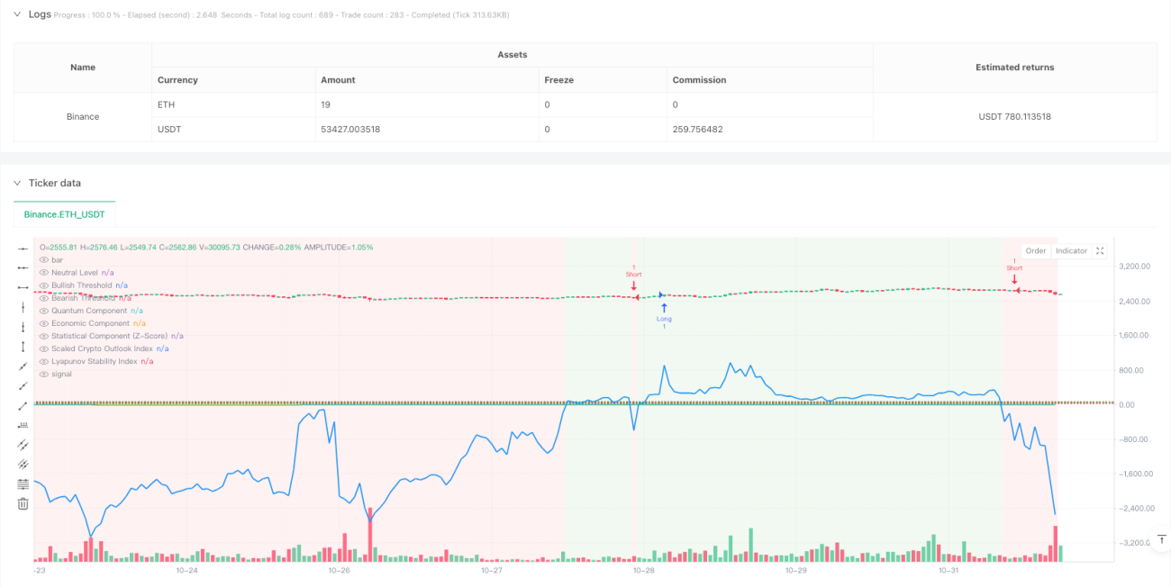
Strategi ini adalah sistem perdagangan kuantitatif inovatif yang menggabungkan prinsip-prinsip mekanika kuantum, statistik dan ekonomi. Ia membina kerangka analisis pasaran yang komprehensif dengan menggabungkan purata bergerak sederhana (SMA), analisis statistik Z-Score, komponen fluktuasi kuantum, indikator dinamik ekonomi dan indeks kestabilan Lyapunov.
Prinsip Strategi
Strategi ini dibina di atas lima tiang teknologi utama:
- Modul analisis statistik menggunakan SMA dan perbezaan piawai untuk mengira Z-Score, menilai kedudukan harga relatif.
- Komponen kuantum mengubah Z-Score menjadi pengayun yang meniru ciri-ciri gelombang keadaan kuantum melalui fungsi indeks dan sinonim.
- Komponen ekonomi menggunakan EMA laju dan perlahan untuk mengukur pergerakan pasaran.
- Indeks Lyapunov menilai keadaan pasaran dengan menganalisis kestabilan gabungan komponen kuantum dan ekonomi.
- Indeks prospek pasaran komprehensif (COI) menggabungkan semua komponen dengan berat yang berbeza untuk membentuk isyarat perdagangan akhir.
Kelebihan Strategik
- Analisis pelbagai dimensi memberikan wawasan pasaran yang lebih menyeluruh dan mengurangkan bias yang mungkin disebabkan oleh satu petunjuk.
- Pengenalan komponen kuantum membawa perspektif yang unik terhadap turun naik pasaran, yang membantu menangkap peluang jangka pendek.
- Penggunaan Indeks Lyapunov berkesan menilai kestabilan pasaran dan meningkatkan keupayaan pengurusan risiko.
- Reka bentuk berat yang boleh disesuaikan membolehkan strategi menyesuaikan diri dengan keadaan pasaran yang berbeza.
- Reka bentuk garisan neutral indeks komprehensif memberikan had isyarat perdagangan yang jelas.
Risiko Strategik
- Tanda-tanda berganda boleh menyebabkan kelewatan isyarat dan menjejaskan masa kemasukan.
- Optimasi parameter yang berlebihan boleh menyebabkan risiko overfitting.
- Dalam pasaran yang bergelombang tinggi, komponen kuantum mungkin menghasilkan isyarat yang terlalu kerap.
- Komponen ekonomi mungkin memberi isyarat yang salah dalam pasaran setapak.
- Penetapan kerugian yang munasabah diperlukan untuk mengawal risiko.
Arah pengoptimuman strategi
- Memperkenalkan sistem berat serasi, menyesuaikan berat komponen mengikut keadaan pasaran yang dinamik.
- Tambah penapis kadar gelombang untuk menyesuaikan sensitiviti isyarat semasa gelombang tinggi.
- Mengintegrasikan indikator sentimen pasaran untuk memberi isyarat tambahan.
- Membangunkan mekanisme hentian kerugian dinamik, menyesuaikan tahap hentian kerugian mengikut keadaan pasaran.
- Tambahkan penapis masa untuk mengelakkan perdagangan pada masa yang tidak menguntungkan.
ringkaskan
Ini adalah strategi perdagangan kuantitatif yang inovatif yang membina kerangka analisis pasaran yang komprehensif dengan menggabungkan teori pelbagai disiplin. Walaupun terdapat beberapa tempat yang perlu dioptimumkan, pendekatan analisis pelbagai dimensi memberikan perspektif yang unik untuk membuat keputusan perdagangan. Dengan pengoptimuman berterusan dan penambahbaikan dalam pengurusan risiko, strategi ini dijangka dapat mengekalkan prestasi yang stabil dalam pelbagai keadaan pasaran.
- 1