
Esta estratégia é baseada na teoria dos níveis de risco de Ben Cowen, com o objetivo de usar os níveis dos bandos BEAM para realizar uma abordagem semelhante. O limite superior do BEAM é a média móvel de 200 semanas após o alinhamento, e o limite inferior é a média móvel de 200 semanas em si. Isso nos dá um alcance de 0 a 1. Quando o preço está abaixo da faixa de 0,5 é emitida uma ordem de compra; Quando o preço está acima da faixa de 0,5 é emitida uma ordem de venda.
A estratégia baseia-se principalmente na teoria de bandas BEAM, proposta por Ben Cowen. Dependendo da variação do preço do BTC, o preço pode ser dividido em 10 áreas entre 0 e 1, que representam 10 níveis de risco diferentes. O nível 0 representa um preço próximo à média móvel de 200 semanas, com o menor risco; o nível 5 representa um preço na zona média; o nível 10 representa um preço próximo à trajetória, com o maior risco.
Quando o preço cai para baixo, a estratégia aumenta gradualmente a posição de compra. Concretamente, se o preço estiver na faixa de 0 a 0,5, uma instrução de compra será emitida em um determinado dia de cada mês definido pela estratégia, e o valor da compra aumentará gradualmente com a diminuição do número da faixa. Por exemplo, na faixa 5, o valor da compra é de 20% do total de DCA do mês; na faixa 1, o valor da compra é aumentado para 100% do total de DCA do mês.
Quando o preço sobe para o nível mais alto, a estratégia diminui gradualmente a posição. Concretamente, se o preço for superior a 0,5 bandas, será emitida uma instrução de venda proporcional, e as posições vendidas serão aumentadas gradualmente com o aumento do número de bandas. Por exemplo, quando a banda 6 for vendida, 6,67%; quando a banda 10 for vendida, todas as posições.
A maior vantagem desta estratégia de média de custo de DCA em bandas de BEAM é que ela aproveita ao máximo as características da negociação de volatilidade do BTC, cobrando posições quando o preço do BTC cai para o mínimo e lucrando quando o preço sobe para o máximo. Esta prática não perde nenhuma boa oportunidade de comprar ou vender.
Em suma, trata-se de uma estratégia de regulação de parâmetros refinada que permite obter ganhos estáveis de longo prazo em situações de turbulência no BTC.
Apesar das vantagens da estratégia de DCA em banda BEAM, existem alguns riscos potenciais que devem ser alertas. Os principais pontos de risco podem ser resumidos como:
Para reduzir os riscos, podem ser tomadas as seguintes medidas:
Considerando os pontos de risco acima, a estratégia pode ser melhorada em:
A estabilidade e a segurança da estratégia podem ser significativamente aumentadas por meio desses meios.
A estratégia de custo médio de DCA da faixa de BEAM é uma estratégia de quantificação de grande valor de combate. Ela usa com sucesso a teoria BEAM para orientar as decisões de negociação e é auxiliada pelo modelo de custo médio para controlar os custos de compra. Ao mesmo tempo, ela também presta atenção ao gerenciamento de riscos, configurando um ponto de parada para evitar a expansão de perdas.
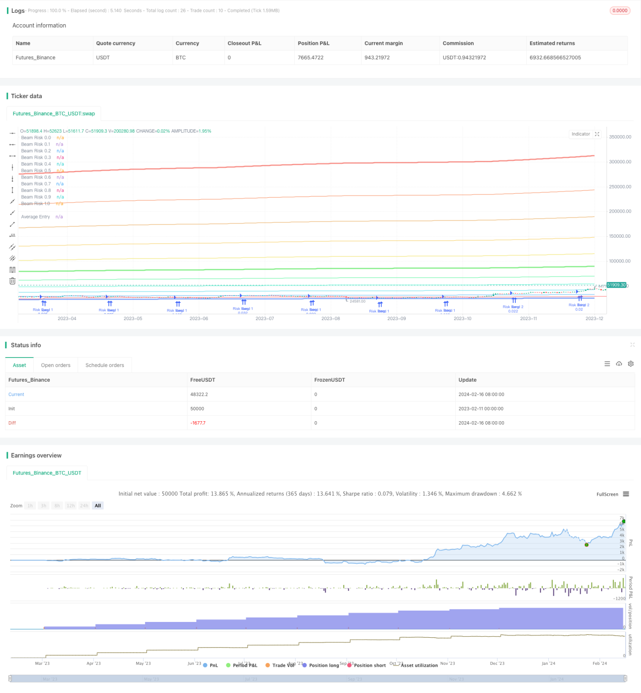
/*backtest
start: 2023-02-11 00:00:00
end: 2024-02-17 00:00:00
period: 1d
basePeriod: 1h
exchanges: [{"eid":"Futures_Binance","currency":"BTC_USDT"}]
*/
// © gjfsdrtytru - BEAM DCA Strategy {
// Based on Ben Cowen's risk level strategy, this aims to copy that method but with BEAM band levels.
// Upper BEAM level is derived from ln(price/200W MA)/2.5, while the 200W MA is the floor price. This is our 0-1 range.
// Buy limit orders are set at the < 0.5 levels and sell orders are set at the > 0.5 level.
//@version=5
strategy(
title = "BEAM DCA Strategy Monthly",
shorttitle = "BEAM DCA M",
overlay = true,
pyramiding = 500,
default_qty_type = strategy.percent_of_equity,
default_qty_value = 0,
initial_capital = 0) //}
// Inputs { ————————————————————————————————————————————————————————————————————
T_ceiling = input.string("Off", "Diminishing Returns", ["Off","Linear","Parabolic"], "Account for diminishing returns as time increases")
day = input.int(1, "DCA Day of Month",1,28,1,"Select day of month for buy orders.")
DCAamount = input.int(1000,"DCA Amount",400,tooltip="Enter the maximum amount you'd be willing to DCA for any given month.")
T_buy = input(true,"Buy Orders","Toggle buy orders.")
T_sell = input(true,"Sell Orders","Toggle sell orders.")
// Time period
testStartYear = input.int(2018, title="Backtest Start Year", minval=2010,maxval=2100,group="Backtest Period")
testStartMonth = input.int(1, title="Backtest Start Month", minval=1, maxval=12, group="Backtest Period")
testStartDay = input.int(1, title="Backtest Start Day", minval=1, maxval=31, group="Backtest Period")
testPeriodLen = input.int(9999, title="Backtest Period (days)", minval=1, group="Backtest Period",tooltip="Days until strategy ends") * 86400000 // convert days into UNIX time
testPeriodStart = timestamp(testStartYear,testStartMonth,testStartDay,0,0)
testPeriodStop = testPeriodStart + testPeriodLen
testPeriod() => true
// ——————————————————————————————————————————————————————————————————————————— }
// Diminishing Returns { ———————————————————————————————————————————————————————
x = bar_index + 1
assetDivisor= 2.5
switch
T_ceiling == "Linear" => assetDivisor:= 3.50542 - 0.000277696 * x
T_ceiling == "Parabolic"=> assetDivisor:= -0.0000001058992338 * math.pow(x,2) + 0.000120729 * x + 3.1982
// ——————————————————————————————————————————————————————————————————————————— }
// Risk Levels { ———————————————————————————————————————————————————————————————
cycleLen = 1400
getMaLen() =>
if bar_index < cycleLen
bar_index + 1
else
cycleLen
// Define Risk Bands
price = close
riskLow = ta.sma(price,getMaLen())
risk1 = riskLow * math.exp((assetDivisor)*0.1)
risk2 = riskLow * math.exp((assetDivisor)*0.2)
risk3 = riskLow * math.exp((assetDivisor)*0.3)
risk4 = riskLow * math.exp((assetDivisor)*0.4)
risk5 = riskLow * math.exp((assetDivisor)*0.5)
risk6 = riskLow * math.exp((assetDivisor)*0.6)
risk7 = riskLow * math.exp((assetDivisor)*0.7)
risk8 = riskLow * math.exp((assetDivisor)*0.8)
risk9 = riskLow * math.exp((assetDivisor)*0.9)
riskHigh = riskLow * math.exp((assetDivisor))
// Plot Risk Bands
p_low = plot(riskLow, "Beam Risk 0.0",color.new(#0042F0,50),3,editable=false)
p_band1 = plot(risk1, "Beam Risk 0.1",color.new(#0090F5,20),1,editable=false)
p_band2 = plot(risk2, "Beam Risk 0.2",color.new(#00C6DB,20),1,editable=false)
p_band3 = plot(risk3, "Beam Risk 0.3",color.new(#00F5BD,20),1,editable=false)
p_band4 = plot(risk4, "Beam Risk 0.4",color.new(#00F069,20),1,editable=false)
p_band5 = plot(risk5, "Beam Risk 0.5",color.new(#00DB08,50),3,editable=false)
p_band6 = plot(risk6, "Beam Risk 0.6",color.new(#E8D20C,20),1,editable=false)
p_band7 = plot(risk7, "Beam Risk 0.7",color.new(#F2B40C,20),1,editable=false)
p_band8 = plot(risk8, "Beam Risk 0.8",color.new(#DC7A00,20),1,editable=false)
p_band9 = plot(risk9, "Beam Risk 0.9",color.new(#F2520C,20),1,editable=false)
p_band10 = plot(riskHigh, "Beam Risk 1.0",color.new(#F01102,50),3,editable=false)
// ——————————————————————————————————————————————————————————————————————————— }
// Order Execution { ———————————————————————————————————————————————————————————
band5 = price<risk5 and price>risk4
band4 = price<risk4 and price>risk3
band3 = price<risk3 and price>risk2
band2 = price<risk2 and price>risk1
band1 = price<risk1
// DCA buy order weights
y = DCAamount / 5
switch
band5 => y:= y * 1
band4 => y:= y * 2
band3 => y:= y * 3
band2 => y:= y * 4
band1 => y:= y * 5
// Contracts per order
contracts =(y/price)
if testPeriod()
// Buy orders
if T_buy == true
if dayofmonth == day
strategy.entry("Risk Band 5",strategy.long,qty=contracts,when=band5)
strategy.entry("Risk Band 4",strategy.long,qty=contracts,when=band4)
strategy.entry("Risk Band 3",strategy.long,qty=contracts,when=band3)
strategy.entry("Risk Band 2",strategy.long,qty=contracts,when=band2)
strategy.entry("Risk Band 1",strategy.long,qty=contracts,when=band1)
// Sell orders
if T_sell == true
if strategy.opentrades > 5
strategy.exit("Risk Band 6",qty_percent=6.67,limit=risk6)
strategy.exit("Risk Band 7",qty_percent=14.28,limit=risk7)
strategy.exit("Risk Band 8",qty_percent=25.00,limit=risk8)
strategy.exit("Risk Band 9",qty_percent=44.44,limit=risk9)
strategy.exit("Risk Band 10",qty_percent=100,limit=riskHigh)
// ——————————————————————————————————————————————————————————————————————————— }
// Info { ——————————————————————————————————————————————————————————————————————
// Line plot of avg. entry price
plot(strategy.position_size > 0 ? strategy.position_avg_price : na,"Average Entry",color.red,trackprice=true,editable=false)
// Unrealised PNL
uPNL = price/strategy.position_avg_price
// Realised PNL
realPNL = 0.
for i = 0 to strategy.closedtrades-1
realPNL += strategy.closedtrades.profit(i)
// Size of open position in ($)
openPosSize = 0.
for i = 0 to strategy.opentrades-1
openPosSize += strategy.opentrades.size(i) * strategy.position_avg_price
// Size of closed position in ($)
closePosSize = 0.
if strategy.closedtrades > 0
for i = 0 to strategy.closedtrades-1
closePosSize += strategy.closedtrades.size(i) * strategy.closedtrades.entry_price(i)
invested = openPosSize+closePosSize // Total capital ($) put into strategy
equity = openPosSize+closePosSize+strategy.openprofit+realPNL // Total current equity ($) in strategy (counting realised PNL)
ROI = (equity-invested) / invested * 100 // ROI of strategy (compare capital invested to excess return)
// // Info Table
// var table table1 = table.new(position.bottom_right,2,9,color.black,color.gray,1,color.gray,2)
// table.cell(table1,0,0,"Capital Invested", text_color=color.white,text_halign=text.align_right)
// table.cell(table1,0,1,"Open Position", text_color=color.white,text_halign=text.align_right)
// table.cell(table1,0,2,"Average Entry", text_color=color.white,text_halign=text.align_right)
// table.cell(table1,0,3,"Last Price", text_color=color.white,text_halign=text.align_right)
// table.cell(table1,0,4,"Open PNL (%)", text_color=color.white,text_halign=text.align_right)
// table.cell(table1,0,5,"Open PNL ($)", text_color=color.white,text_halign=text.align_right)
// table.cell(table1,0,6,"Realised PNL ($)", text_color=color.white,text_halign=text.align_right)
// table.cell(table1,0,7,"Total Equity", text_color=color.white,text_halign=text.align_right)
// table.cell(table1,0,8,"Strategy ROI", text_color=color.white,text_halign=text.align_right)
// table.cell(table1,1,0,"$" + str.tostring(invested, "#,###.00"), text_halign=text.align_right,text_color = color.white)
// table.cell(table1,1,1,"$" + str.tostring(openPosSize, "#,###.00"), text_halign=text.align_right,text_color = color.white)
// table.cell(table1,1,2,"$" + str.tostring(strategy.position_avg_price, "#,###.00"), text_halign=text.align_right,text_color = color.white)
// table.cell(table1,1,3,"$" + str.tostring(price, "#,###.00"), text_halign=text.align_right,text_color = color.white)
// table.cell(table1,1,4, str.tostring((uPNL-1)*100, "#,###.00") + "%",text_halign=text.align_right,text_color = uPNL > 1 ? color.lime : color.red)
// table.cell(table1,1,5,"$" + str.tostring(strategy.openprofit, "#,###.00"), text_halign=text.align_right,text_color = uPNL > 1 ? color.lime : color.red)
// table.cell(table1,1,6,"$" + str.tostring(realPNL, "#,###.00"), text_halign=text.align_right,text_color = color.white)
// table.cell(table1,1,7,"$" + str.tostring(equity, "#,###.00"), text_halign=text.align_right,text_color = color.white)
// table.cell(table1,1,8, str.tostring(ROI, "#,###.00") + "%",text_halign=text.align_right,text_color = ROI > 1 ? color.lime : color.red)
// // ——————————————————————————————————————————————————————————————————————————— }