Indicador de ajuste polinomial do oscilador RSI dinâmico, estratégia de negociação quantitativa

RSI DRSI QR EMA RMSE MSE
Data de criação: 2024-12-11 15:32:23 última modificação: 2024-12-11 15:32:23
cópia: 4 Cliques: 463
1
focar em
1617
Seguidores

Indicador de ajuste polinomial do oscilador RSI dinâmico, estratégia de negociação quantitativa

A estratégia é um sistema de negociação quantitativa baseado em um oscilador dinâmico RSI. A estratégia capta a dinâmica do mercado através da analise de sequência de tempo e de multiplexação do indicador RSI e calcula a taxa de variação do RSI. A estratégia usa métodos matemáticos avançados de processamento de sinais, como a desagregação de QR, e toma decisões de negociação em combinação com o sistema linear uniforme.

Princípio da estratégia

O núcleo da estratégia é o oscilador Delta-RSI, que é implementado através dos seguintes passos:

  1. Em primeiro lugar, calcule o RSI tradicional como base de dados.
  2. O RSI é processado de forma suave, reduzindo o ruído, com o uso de multiple fit
  3. Calcular a variável de tempo do RSI obtendo o delta-RSI, refletindo a taxa de variação do RSI
  4. Comparando o Delta-RSI com sua média móvel para gerar um sinal de negociação
  5. Avaliação e filtragem da qualidade de encaixe com erro de raiz uniforme (RMSE)

Os sinais de transação podem ser gerados de três maneiras:

  • A linha de zero atravessa: Delta-RSI faz mais quando o valor negativo é corrigido, faz zero quando o valor positivo é negativo
  • Linha de sinal de cruzamento: Delta-RSI sobe/baixa em sua média móvel, fazendo um ganho/fraco, respectivamente
  • Mudança de direção: o Delta-RSI faz mais quando a região negativa começa a subir, faz zero quando a região positiva começa a cair

Vantagens estratégicas

  1. Base sólida em matemática: tratamento de sinais com métodos matemáticos avançados, como a decomposição QR, base teórica sólida
  2. Simulação de sinal: a adaptação de múltiplos termos pode filtrar eficazmente o ruído do mercado e melhorar a qualidade do sinal
  3. Flexível: oferece vários modos de geração de sinais e opções de parâmetros para adaptar-se a diferentes ambientes de mercado
  4. Risco controlado: contém um mecanismo de filtragem RMSE, que pode filtrar os sinais de maior confiabilidade
  5. Eficiência de computação: a operação de matrizes usa algoritmos otimizados para operar com maior eficiência

Risco estratégico

  1. Parâmetros sensíveis: vários parâmetros-chave precisam ser cuidadosamente ajustados, e a escolha inadequada de parâmetros pode afetar gravemente a performance da estratégia
  2. Atraso: o processamento suave do sinal pode levar a um certo atraso, podendo perder o processo rápido
  3. Falso breakout: pode gerar falsos sinais e aumentar os custos de transação em mercados turbulentos
  4. Computação complexa: envolve mais operações de matriz e pode haver problemas de desempenho em transações de alta frequência
  5. Super-condicionamento: cuidado é necessário para evitar supercondicionamento de dados históricos ao otimizar os parâmetros

Direção de otimização da estratégia

  1. Parâmetros de auto-adaptação: pode ajustar o ciclo RSI e o número de fases de adaptação de acordo com a dinâmica da volatilidade do mercado
  2. Múltiplos períodos de tempo: sinais com mais períodos de tempo para verificação cruzada
  3. Filtro de taxa de flutuação: adicione indicadores de taxa de flutuação, como o ATR, para filtrar o sinal
  4. Classificação de mercado: diferentes regras de geração de sinais são usadas para diferentes estados de mercado (trend/vibração)
  5. Optimização de stop loss: adição de mecanismos de stop loss mais inteligentes, como stop loss dinâmico baseado em pontos de resistência de suporte

Resumir

Esta é uma estratégia de negociação quantitativa com uma estrutura completa e uma base sólida em teoria. Com a análise das características dinâmicas do RSI, o processamento de sinais em combinação com métodos matemáticos modernos, é possível capturar melhor as tendências do mercado. Embora existam certos problemas de sensibilidade a parâmetros e complexidade de computação, a estratégia tem um bom valor de aplicação com a seleção e otimização razoáveis de parâmetros.
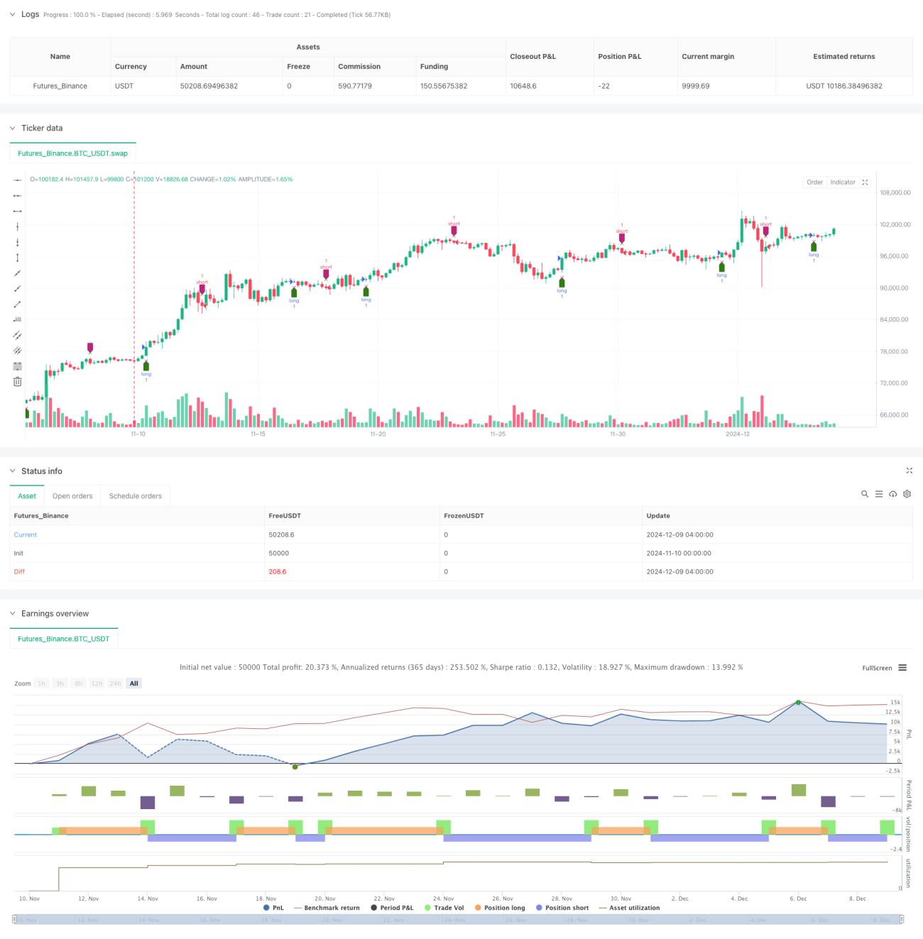
Código-fonte da estratégia
/*backtest
start: 2024-11-10 00:00:00
end: 2024-12-09 08:00:00
period: 4h
basePeriod: 4h
exchanges: [{"eid":"Futures_Binance","currency":"BTC_USDT"}]
*/

// This source code is subject to the terms of the Mozilla Public License 2.0 at https://mozilla.org/MPL/2.0/
// © tbiktag
//
// Delta-RSI Oscillator Strategy
//
// A strategy that uses Delta-RSI Oscillator (© tbiktag) as a stand-alone indicator:
// https://www.tradingview.com/script/OXQVFTQD-Delta-RSI-Oscillator/
//
// Delta-RSI is a smoothed time derivative of the RSI, plotted as a histogram 
// and serving as a momentum indicator. 
// 
// Input parameters:
// RSI Length: The timeframe of the RSI that serves as an input to D-RSI.
// Length: The length of the lookback frame used for local regression.
// Polynomial Order: The order of the local polynomial function used to interpolate the RSI.
// Signal Length: The length of a EMA of the D-RSI series that is used as a signal line.
// Trade signals are generated based on three optional conditions:
// - Zero-crossing: bullish when D-RSI crosses zero from negative to positive values (bearish otherwise)
// - Signal Line Crossing: bullish when D-RSI crosses from below to above the signal line (bearish otherwise)
// - Direction Change: bullish when D-RSI was negative and starts ascending (bearish otherwise)
//
// Since D-RSI oscillator is based on polynomial fitting of the RSI curve, there is also an option
// to filter trade signal by means of the root mean-square error of the fit (normalized by the sample average).
// 
//@version=5
strategy(title='Delta-RSI Oscillator Strategy-QuangVersion', shorttitle='D-RSI-Q', overlay=true)

// ---Subroutines---
matrix_get(_A, _i, _j, _nrows) =>
    // Get the value of the element of an implied 2d matrix
    //input: 
    // _A :: array: pseudo 2d matrix _A = [[column_0],[column_1],...,[column_(n-1)]]
    // _i :: integer: row number
    // _j :: integer: column number
    // _nrows :: integer: number of rows in the implied 2d matrix
    array.get(_A, _i + _nrows * _j)

matrix_set(_A, _value, _i, _j, _nrows) =>
    // Set a value to the element of an implied 2d matrix
    //input: 
    // _A :: array, changed on output: pseudo 2d matrix _A = [[column_0],[column_1],...,[column_(n-1)]]
    // _value :: float: the new value to be set
    // _i :: integer: row number
    // _j :: integer: column number
    // _nrows :: integer: number of rows in the implied 2d matrix
    array.set(_A, _i + _nrows * _j, _value)

transpose(_A, _nrows, _ncolumns) =>
    // Transpose an implied 2d matrix
    // input:
    // _A :: array: pseudo 2d matrix _A = [[column_0],[column_1],...,[column_(n-1)]]
    // _nrows :: integer: number of rows in _A
    // _ncolumns :: integer: number of columns in _A
    // output:
    // _AT :: array: pseudo 2d matrix with implied dimensions: _ncolums x _nrows
    var _AT = array.new_float(_nrows * _ncolumns, 0)
    for i = 0 to _nrows - 1 by 1
        for j = 0 to _ncolumns - 1 by 1
            matrix_set(_AT, matrix_get(_A, i, j, _nrows), j, i, _ncolumns)
    _AT

multiply(_A, _B, _nrowsA, _ncolumnsA, _ncolumnsB) =>
    // Calculate scalar product of two matrices
    // input: 
    // _A :: array: pseudo 2d matrix
    // _B :: array: pseudo 2d matrix
    // _nrowsA :: integer: number of rows in _A
    // _ncolumnsA :: integer: number of columns in _A
    // _ncolumnsB :: integer: number of columns in _B
    // output:
    // _C:: array: pseudo 2d matrix with implied dimensions _nrowsA x _ncolumnsB
    var _C = array.new_float(_nrowsA * _ncolumnsB, 0)
    int _nrowsB = _ncolumnsA
    float elementC = 0.0
    for i = 0 to _nrowsA - 1 by 1
        for j = 0 to _ncolumnsB - 1 by 1
            elementC := 0
            for k = 0 to _ncolumnsA - 1 by 1
                elementC += matrix_get(_A, i, k, _nrowsA) * matrix_get(_B, k, j, _nrowsB)
                elementC
            matrix_set(_C, elementC, i, j, _nrowsA)
    _C

vnorm(_X, _n) =>
    //Square norm of vector _X with size _n
    float _norm = 0.0
    for i = 0 to _n - 1 by 1
        _norm += math.pow(array.get(_X, i), 2)
        _norm
    math.sqrt(_norm)

qr_diag(_A, _nrows, _ncolumns) =>
    //QR Decomposition with Modified Gram-Schmidt Algorithm (Column-Oriented)
    // input:
    // _A :: array: pseudo 2d matrix _A = [[column_0],[column_1],...,[column_(n-1)]]
    // _nrows :: integer: number of rows in _A
    // _ncolumns :: integer: number of columns in _A
    // output:
    // _Q: unitary matrix, implied dimenstions _nrows x _ncolumns
    // _R: upper triangular matrix, implied dimansions _ncolumns x _ncolumns
    var _Q = array.new_float(_nrows * _ncolumns, 0)
    var _R = array.new_float(_ncolumns * _ncolumns, 0)
    var _a = array.new_float(_nrows, 0)
    var _q = array.new_float(_nrows, 0)
    float _r = 0.0
    float _aux = 0.0
    //get first column of _A and its norm:
    for i = 0 to _nrows - 1 by 1
        array.set(_a, i, matrix_get(_A, i, 0, _nrows))
    _r := vnorm(_a, _nrows)
    //assign first diagonal element of R and first column of Q
    matrix_set(_R, _r, 0, 0, _ncolumns)
    for i = 0 to _nrows - 1 by 1
        matrix_set(_Q, array.get(_a, i) / _r, i, 0, _nrows)
    if _ncolumns != 1
        //repeat for the rest of the columns
        for k = 1 to _ncolumns - 1 by 1
            for i = 0 to _nrows - 1 by 1
                array.set(_a, i, matrix_get(_A, i, k, _nrows))
            for j = 0 to k - 1 by 1
                //get R_jk as scalar product of Q_j column and A_k column:
                _r := 0
                for i = 0 to _nrows - 1 by 1
                    _r += matrix_get(_Q, i, j, _nrows) * array.get(_a, i)
                    _r
                matrix_set(_R, _r, j, k, _ncolumns)
                //update vector _a
                for i = 0 to _nrows - 1 by 1
                    _aux := array.get(_a, i) - _r * matrix_get(_Q, i, j, _nrows)
                    array.set(_a, i, _aux)
            //get diagonal R_kk and Q_k column
            _r := vnorm(_a, _nrows)
            matrix_set(_R, _r, k, k, _ncolumns)
            for i = 0 to _nrows - 1 by 1
                matrix_set(_Q, array.get(_a, i) / _r, i, k, _nrows)
    [_Q, _R]

pinv(_A, _nrows, _ncolumns) =>
    //Pseudoinverse of matrix _A calculated using QR decomposition
    // Input: 
    // _A:: array: implied as a (_nrows x _ncolumns) matrix _A = [[column_0],[column_1],...,[column_(_ncolumns-1)]]
    // Output: 
    // _Ainv:: array implied as a (_ncolumns x _nrows) matrix _A = [[row_0],[row_1],...,[row_(_nrows-1)]]
    // ----
    // First find the QR factorization of A: A = QR,
    // where R is upper triangular matrix.
    // Then _Ainv = R^-1*Q^T.
    // ----
    [_Q, _R] = qr_diag(_A, _nrows, _ncolumns)
    _QT = transpose(_Q, _nrows, _ncolumns)
    // Calculate Rinv:
    var _Rinv = array.new_float(_ncolumns * _ncolumns, 0)
    float _r = 0.0
    matrix_set(_Rinv, 1 / matrix_get(_R, 0, 0, _ncolumns), 0, 0, _ncolumns)
    if _ncolumns != 1
        for j = 1 to _ncolumns - 1 by 1
            for i = 0 to j - 1 by 1
                _r := 0.0
                for k = i to j - 1 by 1
                    _r += matrix_get(_Rinv, i, k, _ncolumns) * matrix_get(_R, k, j, _ncolumns)
                    _r
                matrix_set(_Rinv, _r, i, j, _ncolumns)
            for k = 0 to j - 1 by 1
                matrix_set(_Rinv, -matrix_get(_Rinv, k, j, _ncolumns) / matrix_get(_R, j, j, _ncolumns), k, j, _ncolumns)
            matrix_set(_Rinv, 1 / matrix_get(_R, j, j, _ncolumns), j, j, _ncolumns)
    //
    _Ainv = multiply(_Rinv, _QT, _ncolumns, _ncolumns, _nrows)
    _Ainv

norm_rmse(_x, _xhat) =>
    // Root Mean Square Error normalized to the sample mean
    // _x.   :: array float, original data
    // _xhat :: array float, model estimate
    // output
    // _nrmse:: float
    float _nrmse = 0.0
    if array.size(_x) != array.size(_xhat)
        _nrmse := na
        _nrmse
    else
        int _N = array.size(_x)
        float _mse = 0.0
        for i = 0 to _N - 1 by 1
            _mse += math.pow(array.get(_x, i) - array.get(_xhat, i), 2) / _N
            _mse
        _xmean = array.sum(_x) / _N
        _nrmse := math.sqrt(_mse) / _xmean
        _nrmse
    _nrmse


diff(_src, _window, _degree) =>
    // Polynomial differentiator
    // input:
    // _src:: input series
    // _window:: integer: wigth of the moving lookback window
    // _degree:: integer: degree of fitting polynomial
    // output:
    // _diff :: series: time derivative
    // _nrmse:: float: normalized root mean square error
    //
    // Vandermonde matrix with implied dimensions (window x degree+1)
    // Linear form: J = [ [z]^0, [z]^1, ... [z]^degree], with z = [ (1-window)/2 to (window-1)/2 ] 
    var _J = array.new_float(_window * (_degree + 1), 0)
    for i = 0 to _window - 1 by 1
        for j = 0 to _degree by 1
            matrix_set(_J, math.pow(i, j), i, j, _window)
    // Vector of raw datapoints:
    var _Y_raw = array.new_float(_window, na)
    for j = 0 to _window - 1 by 1
        array.set(_Y_raw, j, _src[_window - 1 - j])
    // Calculate polynomial coefficients which minimize the loss function
    _C = pinv(_J, _window, _degree + 1)
    _a_coef = multiply(_C, _Y_raw, _degree + 1, _window, 1)
    // For first derivative, approximate the last point (i.e. z=window-1) by 
    float _diff = 0.0
    for i = 1 to _degree by 1
        _diff += i * array.get(_a_coef, i) * math.pow(_window - 1, i - 1)
        _diff
    // Calculates data estimate (needed for rmse)
    _Y_hat = multiply(_J, _a_coef, _window, _degree + 1, 1)
    float _nrmse = norm_rmse(_Y_raw, _Y_hat)
    [_diff, _nrmse]

/// --- main ---
degree = input.int(title='Polynomial Order', group='Model Parameters:', inline='linepar1', defval=2, minval=1)
rsi_l = input.int(title='RSI Length', group='Model Parameters:', inline='linepar1', defval=21, minval=1, tooltip='The period length of RSI that is used as input.')
window = input.int(title='Length ( > Order)', group='Model Parameters:', inline='linepar2', defval=21, minval=2)
signalLength = input.int(title='Signal Length', group='Model Parameters:', inline='linepar2', defval=9, tooltip='The signal line is a EMA of the D-RSI time series.')
islong = input.bool(title='Buy', group='Show Signals:', inline='lineent', defval=true)
isshort = input.bool(title='Sell', group='Show Signals:', inline='lineent', defval=true)
showendlabels = input.bool(title='Exit', group='Show Signals:', inline='lineent', defval=true)
buycond = input.string(title='Buy', group='Entry and Exit Conditions:', inline='linecond', defval='Zero-Crossing', options=['Zero-Crossing', 'Signal Line Crossing', 'Direction Change'])
sellcond = input.string(title='Sell', group='Entry and Exit Conditions:', inline='linecond', defval='Zero-Crossing', options=['Zero-Crossing', 'Signal Line Crossing', 'Direction Change'])
endcond = input.string(title='Exit', group='Entry and Exit Conditions:', inline='linecond', defval='Zero-Crossing', options=['Zero-Crossing', 'Signal Line Crossing', 'Direction Change'])
usenrmse = input.bool(title='', group='Filter by Means of Root-Mean-Square Error of RSI Fitting:', inline='linermse', defval=false)
rmse_thrs = input.float(title='RSI fitting Error Threshold, %', group='Filter by Means of Root-Mean-Square Error of RSI Fitting:', inline='linermse', defval=10, minval=0.0) / 100


src = ta.rsi(close, rsi_l)
[drsi, nrmse] = diff(src, window, degree)
signalline = ta.ema(drsi, signalLength)

// Conditions and filters
filter_rmse = usenrmse ? nrmse < rmse_thrs : true
dirchangeup = drsi > drsi[1] and drsi[1] < drsi[2] and drsi[1] < 0.0
dirchangedw = drsi < drsi[1] and drsi[1] > drsi[2] and drsi[1] > 0.0
crossup = ta.crossover(drsi, 0.0)
crossdw = ta.crossunder(drsi, 0.0)
crosssignalup = ta.crossover(drsi, signalline)
crosssignaldw = ta.crossunder(drsi, signalline)

//Signals
golong = (buycond == 'Direction Change' ? dirchangeup : buycond == 'Zero-Crossing' ? crossup : crosssignalup) and filter_rmse
goshort = (sellcond == 'Direction Change' ? dirchangedw : sellcond == 'Zero-Crossing' ? crossdw : crosssignaldw) and filter_rmse
endlong = (endcond == 'Direction Change' ? dirchangedw : endcond == 'Zero-Crossing' ? crossdw : crosssignaldw) and filter_rmse
endshort = (endcond == 'Direction Change' ? dirchangeup : endcond == 'Zero-Crossing' ? crossup : crosssignalup) and filter_rmse
plotshape(golong and islong ? low : na, location=location.belowbar, style=shape.labelup, color=color.new(#2E7C13, 0), size=size.small, title='Buy')
plotshape(goshort and isshort ? high : na, location=location.abovebar, style=shape.labeldown, color=color.new(#BF217C, 0), size=size.small, title='Sell')
plotshape(showendlabels and endlong and islong ? high : na, location=location.abovebar, style=shape.xcross, color=color.new(#2E7C13, 0), size=size.tiny, title='Exit Long')
plotshape(showendlabels and endshort and isshort ? low : na, location=location.belowbar, style=shape.xcross, color=color.new(#BF217C, 0), size=size.tiny, title='Exit Short')

alertcondition(golong, title='Long Signal', message='D-RSI: Long Signal')
alertcondition(goshort, title='Short Signal', message='D-RSI: Short Signal')
alertcondition(endlong, title='Exit Long Signal', message='D-RSI: Exit Long')
alertcondition(endshort, title='Exit Short Signal', message='D-RSI: Exit Short')

strategy.entry('long', strategy.long, when=golong and islong)
strategy.entry('short', strategy.short, when=goshort and isshort)
strategy.close('long', when=endlong and islong)
strategy.close('short', when=endshort and isshort)