
Por que os indicadores tecnológicos tradicionais falham em mercados complexos?
Na área de negociação quantitativa, muitas vezes enfrentamos um problema central: um único indicador técnico é propenso a produzir falsos sinais em meio ao ruído do mercado, levando a frequentes paradas e retiradas de capital. Então, como construir um sistema de negociação que capte tendências e filtre o ruído de forma eficaz?
A estratégia de filtragem múltipla do canal de Gauss, analisada hoje, oferece-nos uma solução digna de aprofundamento através da combinação de quatro indicadores técnicos de diferentes dimensões.
Arquitetura Tecnológica do Núcleo: Como os quatro filtros funcionam em conjunto?
1. Gaussian Channel - Identificação de tendências
A base da estratégia é um filtro de Gauss de 4 níveis, com uma janela de amostragem de 144 ciclos. Ao contrário da média móvel tradicional, o filtro de Gauss elimina a maior parte do ruído do mercado através da modelagem matemática, mantendo a sensibilidade às mudanças de preço.
Parâmetros-chave:
- Número de pontos de Gauss: 4 (equilibrando retardo e suavidade)
- Período de amostragem: 144 (para capturar tendências de médio prazo)
- Multiplicador de filtro: 1.414 (multiplicador de diferença padrão, controle de largura do canal)
2. Linha Kijun-Sen ((130 ciclos) - Confirmação de tendências de médio e longo prazo
A linha Kijun-Sen de 130 ciclos é usada como filtro de tendência, em vez dos tradicionais 26 ciclos. Qual é a importância desse ajuste?
A configuração de ciclo mais longo permite:
- Redução de falsos sinais de ruptura
- Assegurar que a direção das transações esteja de acordo com as principais tendências
- Melhorar a qualidade do sinal e reduzir a frequência das transações
3. Indicador VAPI - Análise de preços de volume de transação
VAPI (Volume Adjusted Price Indicator) é um indicador de volume ajustado que analisa a relação entre volume de transação e mudanças de preço para determinar a verdadeira intenção dos participantes do mercado. Quando o VAPI é > 0, o suporte é excessivo e quando é < 0, o suporte é vazio.
4. ATR Dynamic Stop Loss - Mecanismo de Controle de Risco
Usando 4,5 vezes o ATR de 11 ciclos como distância de parada, essa configuração considera a volatilidade do mercado e evita que a parada seja muito apertada e desencadeada pelo ruído do mercado.
Inovação na gestão de fundos: a sabedoria da estratégia de divisão 75/25
O que mais vale a pena aprender com esta estratégia é a sua maneira única de administrar o dinheiro:
Logística de distribuição:
- 75% de posições: fixação de 3,5 vezes o risco de retorno do que o stop loss
- 25% de posições: traçado dinâmico de stop loss
Por que isso?
- Garantir o rendimento básicoA paralisação de 75% das posições garantiu um retorno estável para a maioria dos investimentos.
- Capturar o excesso de receitaPerda de seguimento de 25% de posições permite obter maiores ganhos se a tendência continuar
- Dispersão de riscosA diferença de mecanismos de saída diminui o risco de uma única estratégia falhar
Sistemas de controlo de riscos: mecanismos de proteção em vários níveis
1. Controle de risco de entrada
- O risco de cada transação é limitado a 3% do capital da conta
- Cálculo de posições dinâmicas baseado no ATR
2. Gerenciamento de riscos de detenção
- Prejuízo principal: 4,5 vezes o ATR
- Perda de rastreamento: ajuste dinâmico, bloqueio de flutuação
- Proteção adicional: 10% de proteção de receita fixa
3. Mecanismo de filtragem de sinal
Os quatro indicadores técnicos foram simultaneamente confirmados, reduzindo significativamente a probabilidade de falsos sinais.
Análise de vantagens e limitações estratégicas
Os principais pontos fortes:
- Qualidade de sinalO mecanismo de filtragem múltipla aumenta significativamente a confiabilidade dos sinais de transação.
- Riscos controladosSistema perfeito de gestão de stop loss e posições
- Altamente adaptávelATR: Dinâmica de ajustes para adaptar-se a diferentes ambientes de mercado
- Otimização de receitasA estratégia de divisão de posições equilibra os ganhos estáveis com os excedentes.
Limites potenciais:
- Dependência de tendênciaO que é que os investidores estão a fazer?
- Parâmetros sensíveisOs vários parâmetros precisam ser otimizados para diferentes variedades:
- AtrasoA falta de filtragem pode atrasar a entrada.
Recomendações para aplicações em combate
1. Seleção de variedades
Preferência para variedades com forte tendência, como os principais pares de moedas, futuros de índices de ações, etc.
Optimização de parâmetros 2.
Recomenda-se que o retrospecto seja otimizado com base nos dados históricos das variedades de transação específicas, com especial atenção para:
- Ciclo de amostragem do Canal de Gauss
- Período de Kijun-Sen
- ATR Stop Loss Multiplier
3. Adaptação ao mercado
Em mercados com uma visível oscilação, pode-se considerar a suspensão da estratégia ou ajustar a configuração dos parâmetros.
Resumo: Pensamento sistêmico em transações quantitativas
O valor desta estratégia não está apenas na sua implementação técnica, mas na sua forma de pensar sistematicamente:
- Verificação multidimensionalVerificar sinais de negociação de várias perspectivas, como tendência, volume de transação e volatilidade
- Prioridade ao riscoA base da estratégia é um bom sistema de controlo de riscos
- Otimização de receitasA estratégia de divisão de posições equilibra diferentes objetivos de lucro.
A estratégia fornece um bom referencial de estrutura para os comerciantes de quantidade. A chave não é seguir os parâmetros, mas entender a sua concepção e fazer ajustes adequados de acordo com a sua própria variedade de negociação e preferências de risco.
Lembre-se que a melhor estratégia não é a mais complexa, mas a que melhor se adequa ao seu estilo de negociação e ao seu ambiente de mercado.
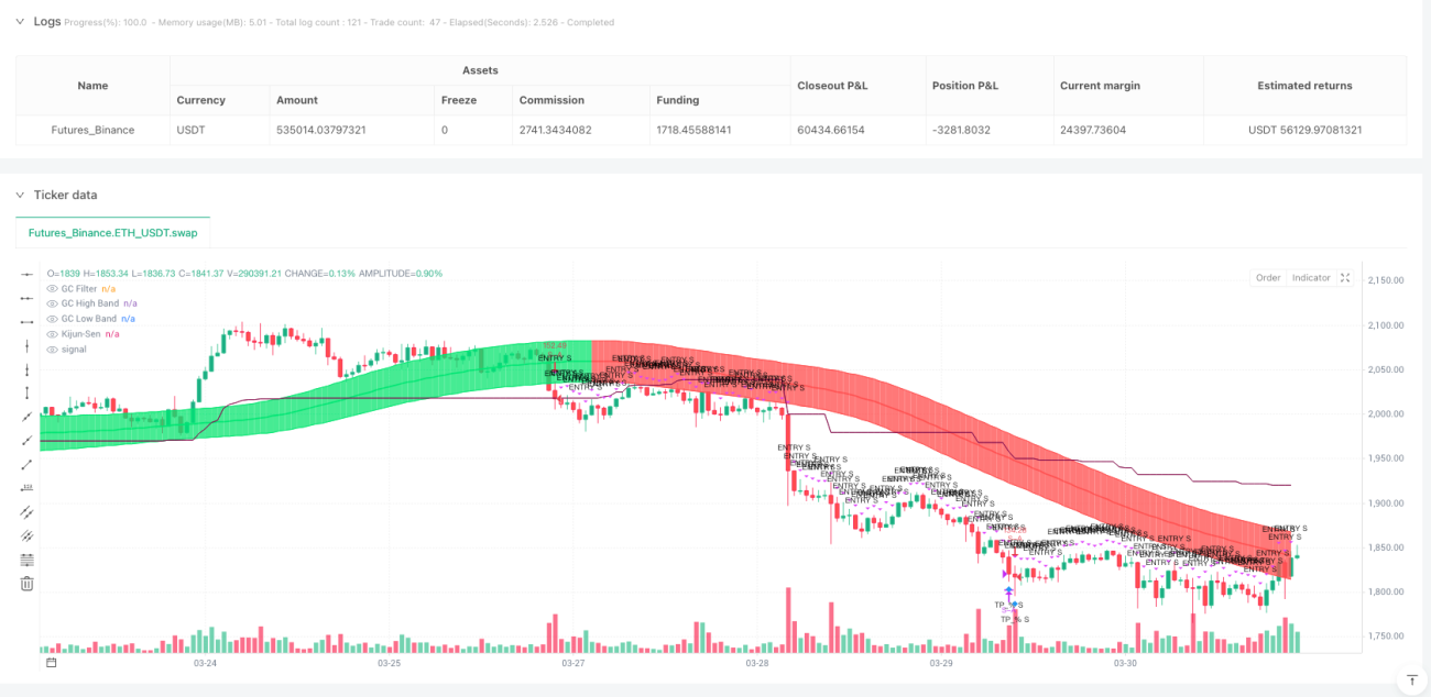
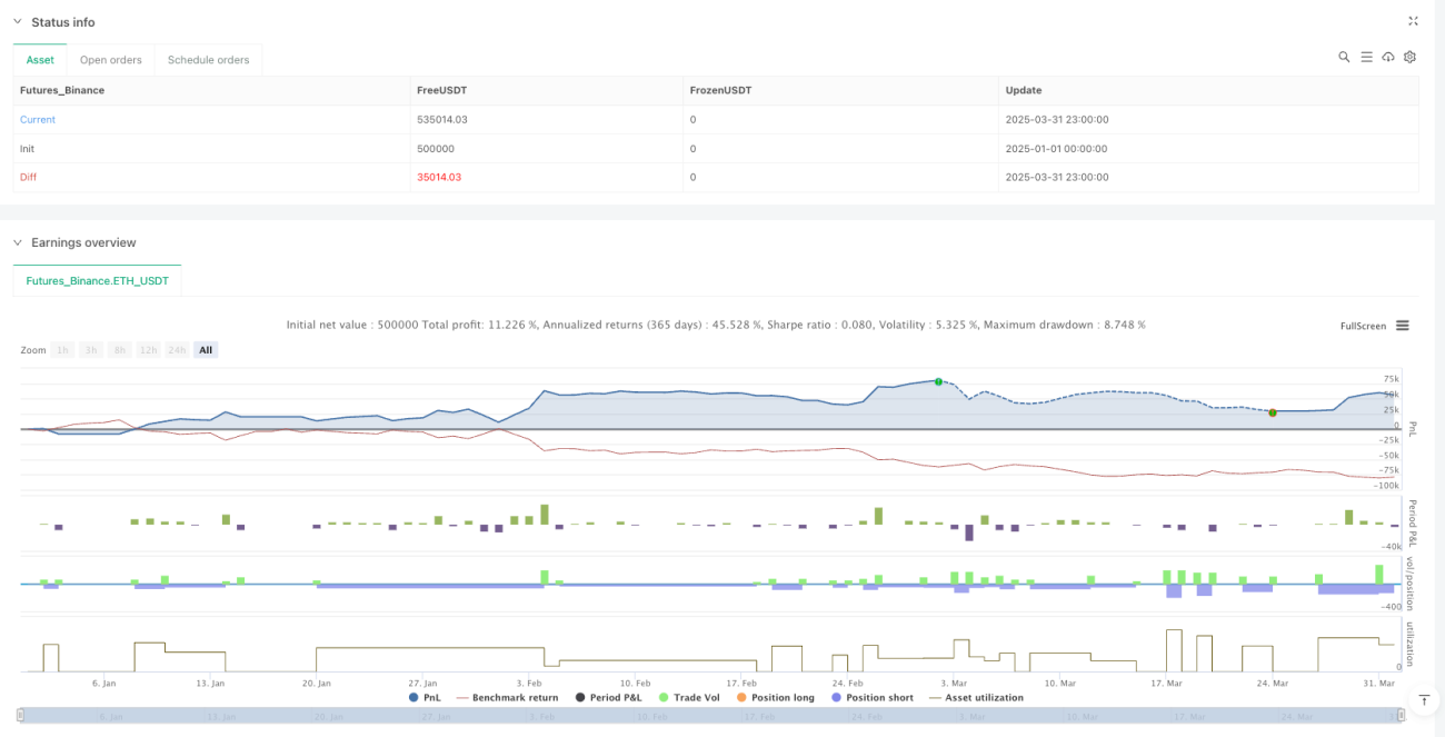
/*backtest
start: 2025-01-01 00:00:00
end: 2025-04-01 00:00:00
period: 1h
basePeriod: 1h
exchanges: [{"eid":"Futures_Binance","currency":"ETH_USDT","balance":500000}]
*/

// @version=6
strategy("Gaussian Channel Strategy – GC + Kijun (120) + VAPI Gate + ATR(4.5x) + 75/25 TP-TRAIL + Extra %TP",
     overlay=true)
- 1