
Tổng quan
Chiến lược này là một hệ thống giao dịch theo dõi xu hướng dựa trên Gaussian Ripple và StochRSI. Chiến lược này sử dụng Gaussian Channel để xác định xu hướng thị trường và kết hợp với StochRSI để tối ưu hóa thời gian vào. Hệ thống sử dụng phương pháp kết hợp đa phương thức để xây dựng Gaussian Channel, theo dõi xu hướng giá bằng cách điều chỉnh động lực của quỹ đạo lên xuống, để theo dõi chính xác xu hướng thị trường.
Nguyên tắc chiến lược
Nền tảng của chiến lược là một kênh giá được xây dựng dựa trên thuật toán Goslin Wave. Thực hiện cụ thể bao gồm một số bước quan trọng sau:
- Sử dụng hàm đa thức f_filt9x để thực hiện các sóng Gaussian bậc 9 để cải thiện hiệu quả của các sóng Gaussian bằng cách tối ưu hóa cực
- Đường sóng chính và kênh tỷ lệ dao động dựa trên giá HLC3
- Khởi động chế độ giảm Lag để giảm độ trễ của vibrator, chế độ FastResponse để tăng tốc độ đáp ứng
- Sử dụng chỉ số StochRSI để xác định tín hiệu giao dịch trong phạm vi mua và bán quá mức ((80/20)
- Tăng đường Gauss và giá phá vỡ đường ray, kết hợp với chỉ số StochRSI tạo ra tín hiệu đa
- Bán ngay khi giá giảm xuống đường
Lợi thế chiến lược
- Gaussian có khả năng giảm tiếng ồn tốt, có thể lọc hiệu quả tiếng ồn thị trường
- Theo dõi xu hướng trơn tru, giảm tín hiệu sai
- Hỗ trợ tối ưu hóa độ trễ và mô hình phản ứng nhanh, có thể điều chỉnh linh hoạt theo đặc điểm thị trường
- Kết hợp với chỉ số StochRSI để tối ưu hóa thời gian đầu vào và tăng tỷ lệ giao dịch thành công
- Sử dụng chiều rộng kênh động để thích ứng với sự biến động của thị trường
Rủi ro chiến lược
- Có một số sự chậm trễ của Gauss, có thể dẫn đến việc nhập cảnh hoặc xuất cảnh không kịp thời
- Có thể tạo ra các tín hiệu giao dịch thường xuyên trong thị trường bất ổn, làm tăng chi phí giao dịch
- StochRSI có thể tạo ra tín hiệu tụt hậu trong một số điều kiện thị trường
- Quá trình tối ưu hóa tham số phức tạp, cần điều chỉnh lại các tham số cho các môi trường thị trường khác nhau
- Hệ thống có yêu cầu về tài nguyên tính toán cao, tính toán thời gian thực có một số độ trễ
Hướng tối ưu hóa chiến lược
- Tiến hành cơ chế tối ưu hóa tham số thích ứng, điều chỉnh tham số theo tình trạng thị trường động
- Thêm mô-đun nhận diện môi trường thị trường, sử dụng các tham số khác nhau trong các điều kiện thị trường khác nhau
- Tối ưu hóa thuật toán Gosselin để giảm thêm độ trễ tính toán
- Nhập nhiều chỉ số kỹ thuật để kiểm tra chéo và tăng độ tin cậy tín hiệu
- Phát triển cơ chế dừng lỗ thông minh, nâng cao khả năng kiểm soát rủi ro
Tóm tắt
Chiến lược này có khả năng theo dõi hiệu quả các xu hướng thị trường thông qua sự kết hợp của các chỉ số Gaussian và StochRSI. Hệ thống có khả năng giảm tiếng ồn và nhận biết xu hướng tốt, nhưng cũng có một số độ trì trệ và khó tối ưu hóa tham số. Bằng cách tối ưu hóa và hoàn thiện liên tục, chiến lược này có thể đạt được lợi nhuận ổn định trong giao dịch thực tế.
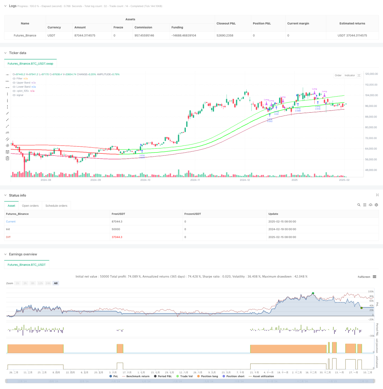
/*backtest
start: 2024-02-19 00:00:00
end: 2025-02-16 08:00:00
period: 1d
basePeriod: 1d
exchanges: [{"eid":"Futures_Binance","currency":"BTC_USDT"}]
*/

//@version=5
strategy(title="Demo GPT - Gaussian Channel Strategy v3.0", overlay=true, commission_type=strategy.commission.percent, commission_value=0.1, slippage=0, default_qty_type=strategy.percent_of_equity, default_qty_value=250)

// ============================================- 1