Chiến lược giao dịch động lượng đa chiều dựa trên phân tích quang phổ lượng tử

Tổng quan
Chiến lược này là một hệ thống giao dịch định lượng sáng tạo kết hợp các nguyên tắc của cơ học lượng tử, thống kê và kinh tế. Nó xây dựng một khuôn khổ phân tích thị trường toàn diện bằng cách kết hợp trung bình di chuyển đơn giản (SMA), phân tích thống kê Z-Score, thành phần dao động lượng tử, chỉ số động lực kinh tế và chỉ số ổn định của Lyapunov.
Nguyên tắc chiến lược
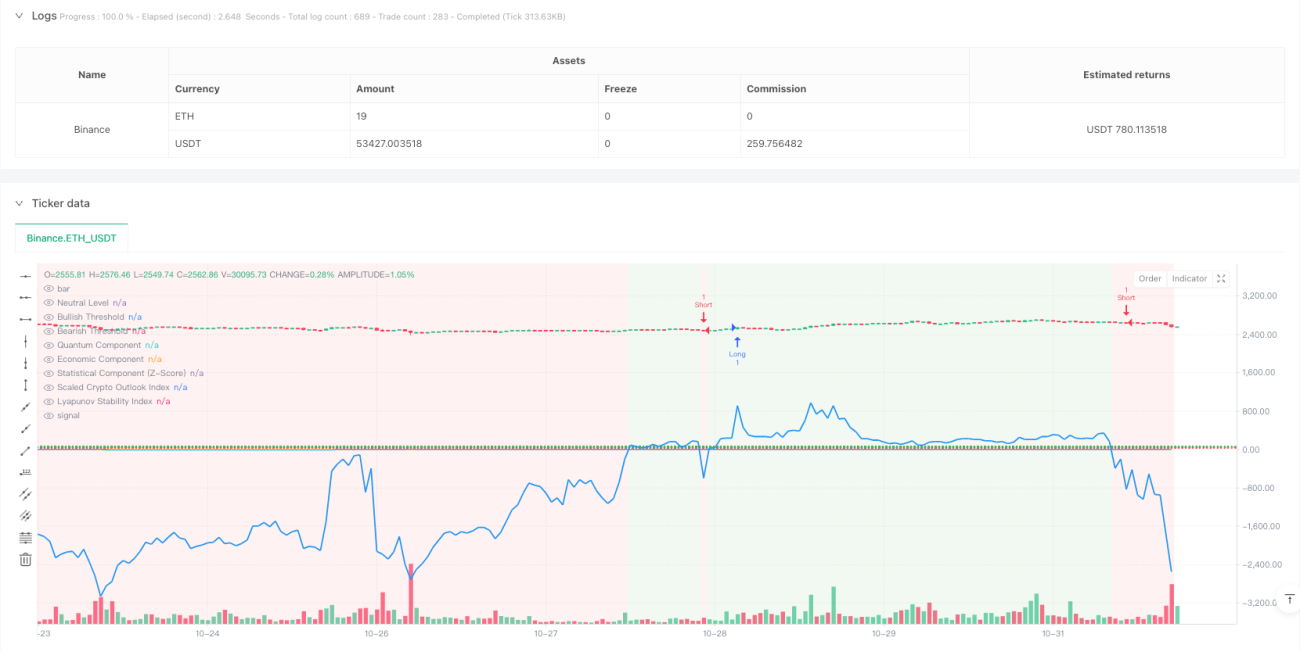
Chiến lược được xây dựng dựa trên năm trụ cột kỹ thuật chính:
- Mô-đun phân tích thống kê sử dụng SMA và chênh lệch chuẩn để tính toán Z-Score, đánh giá vị trí tương đối của giá.
- Bộ phận lượng tử chuyển đổi Z-Score thành một dao động, mô phỏng tính chất dao động của trạng thái lượng tử thông qua hàm số và hàm âm.
- Thành phần kinh tế sử dụng tỷ lệ đối số của EMA nhanh và chậm để đo động lực thị trường.
- Chỉ số Lyapunov đánh giá tình trạng thị trường bằng cách phân tích sự ổn định kết hợp của các thành phần lượng tử và kinh tế.
- Chỉ số triển vọng thị trường tổng hợp (COI) kết hợp tất cả các thành phần theo trọng lượng khác nhau để tạo thành tín hiệu giao dịch cuối cùng.
Lợi thế chiến lược
- Phân tích đa chiều cung cấp một cái nhìn toàn diện hơn về thị trường, giảm sự sai lệch mà chỉ số đơn lẻ có thể mang lại.
- Việc giới thiệu các thành phần lượng tử mang lại một viễn cảnh biến động thị trường độc đáo, giúp nắm bắt các cơ hội ngắn hạn.
- Việc sử dụng chỉ số Lyapunov có thể đánh giá hiệu quả sự ổn định của thị trường và cải thiện khả năng quản lý rủi ro.
- Thiết kế có thể điều chỉnh trọng lượng cho phép chiến lược thích ứng linh hoạt với các môi trường thị trường khác nhau.
- Thiết kế đường trung tính của chỉ số tổng hợp cung cấp ranh giới tín hiệu giao dịch rõ ràng.
Rủi ro chiến lược
- Nhiều chỉ số có thể gây ra sự chậm trễ tín hiệu, ảnh hưởng đến thời gian nhập cảnh.
- Các tham số được tối ưu hóa quá mức có thể dẫn đến nguy cơ quá phù hợp.
- Trong thị trường có biến động cao, các bộ phận lượng tử có thể tạo ra các tín hiệu quá thường xuyên.
- Các thành phần kinh tế có thể tạo ra tín hiệu sai lệch trong thị trường ngang.
- Cần thiết lập mức dừng lỗ hợp lý để kiểm soát rủi ro.
Hướng tối ưu hóa chiến lược
- Tiến hành hệ thống trọng lượng thích ứng, điều chỉnh trọng lượng của các thành phần theo động lực của môi trường thị trường.
- Tăng bộ lọc tần số dao động, điều chỉnh độ nhạy của tín hiệu trong thời gian dao động cao.
- Kết hợp các chỉ số cảm xúc thị trường để cung cấp tín hiệu xác nhận bổ sung.
- Phát triển cơ chế dừng lỗ động, điều chỉnh mức dừng lỗ theo điều kiện thị trường.
- Thêm một bộ lọc thời gian để tránh đặt hàng vào thời điểm giao dịch không thuận lợi.
Tóm tắt
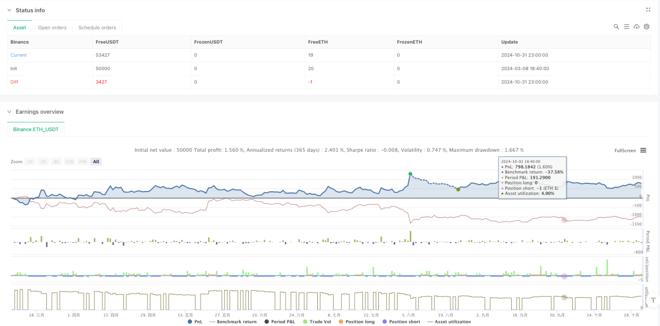
Đây là một chiến lược giao dịch định lượng sáng tạo, xây dựng một khuôn khổ phân tích thị trường toàn diện bằng cách kết hợp lý thuyết đa ngành. Mặc dù có một số nơi cần được tối ưu hóa, phương pháp phân tích đa chiều của nó cung cấp một góc nhìn độc đáo cho quyết định giao dịch. Bằng cách cải thiện liên tục tối ưu hóa và quản lý rủi ro, chiến lược này dự kiến sẽ duy trì hiệu suất ổn định trong các môi trường thị trường khác nhau.
- 1