Chiến lược giao dịch tích hợp đa chiều dựa trên Nadaraya-Watson

SMA RSI ATR
Ngày tạo: 2025-02-20 17:38:44 sửa đổi lần cuối: 2025-02-27 17:21:26
sao chép: 0 Số nhấp chuột: 446
2
tập trung vào
319
Người theo dõi

Chiến lược giao dịch tích hợp đa chiều dựa trên Nadaraya-Watson Chiến lược giao dịch tích hợp đa chiều dựa trên Nadaraya-Watson

Tổng quan

Chiến lược này là một hệ thống giao dịch đa chiều dựa trên Nadaraya-Watson Nuclear Regression, tạo thành tín hiệu tổng hợp để hướng dẫn quyết định giao dịch bằng cách tích hợp thông tin thị trường về bốn chiều kỹ thuật, cảm xúc, siêu cảm giác và ý định. Chiến lược sử dụng phương pháp tối ưu hóa trọng lượng, xử lý trọng lượng các tín hiệu ở các chiều khác nhau và kết hợp các bộ lọc xu hướng và động lực để nâng cao chất lượng tín hiệu.

Nguyên tắc chiến lược

Cốt lõi của chiến lược là xử lý trơn tru dữ liệu thị trường đa chiều thông qua phương pháp thu hồi hạt nhân Nadaraya-Watson. Cụ thể:

  1. Kích thước kỹ thuật sử dụng giá đóng cửa
  2. Dimension cảm xúc sử dụng chỉ số RSI
  3. Tỷ lệ dao động của ATR
  4. Giá sử dụng chiều hướng và độ lệch đường trung bình Sau khi các chiều này được làm mịn trở lại hạt nhân, chúng được tích hợp trọng lượng bằng trọng lượng đặt trước ((công nghệ 0.4, cảm xúc 0.2, siêu cảm xúc 0.2, ý định 0.2) để tạo thành tín hiệu giao dịch cuối cùng. Khi tín hiệu tích hợp và đường trung bình di chuyển của nó xảy ra, lệnh giao dịch được phát hành sau khi xác nhận theo xu hướng và bộ lọc động lượng.

Lợi thế chiến lược

  1. Phân tích đa chiều cung cấp cái nhìn toàn diện hơn về thị trường, tránh những hạn chế của chỉ số đơn lẻ
  2. Nadaraya-Watson Nuclear Regression có thể làm giảm tiếng ồn thị trường và cung cấp tín hiệu mượt mà hơn
  3. Cơ chế tối ưu hóa trọng lượng cho phép điều chỉnh tầm quan trọng của các chiều tùy theo đặc điểm thị trường
  4. Thêm bộ lọc xu hướng và động lực đã cải thiện đáng kể chất lượng tín hiệu
  5. Hệ thống quản lý rủi ro tốt đảm bảo an toàn tài chính

Rủi ro chiến lược

  1. Tối ưu hóa tham số quá mức có thể dẫn đến quá khớp
  2. Điều kiện lọc đa có thể bỏ qua một số tín hiệu hiệu quả
  3. Tính phức tạp của tính toán hồi quy hạt nhân có thể ảnh hưởng đến hiệu suất thời gian thực
  4. Phân phối trọng lượng không đúng đắn có thể làm suy yếu một số tín hiệu thị trường quan trọng Các biện pháp giảm thiểu bao gồm: sử dụng tham số xác thực thử nghiệm ngoài mẫu, điều chỉnh các điều kiện lọc động, tối ưu hóa hiệu quả tính toán, đánh giá thường xuyên và điều chỉnh phân bổ trọng lượng.

Hướng tối ưu hóa chiến lược

  1. Tiến hành hệ thống trọng lượng thích ứng, điều chỉnh trọng lượng theo các chiều theo tình hình thị trường
  2. Phát triển cơ chế lọc thông minh hơn, cân bằng chất lượng và số lượng tín hiệu
  3. Tối ưu hóa thực hiện thuật toán Nadaraya-Watson để cải thiện hiệu quả tính toán
  4. Thêm mô-đun nhận dạng chu kỳ thị trường, thiết lập tham số khác nhau trong các giai đoạn thị trường khác nhau
  5. Mở rộng hệ thống quản lý rủi ro, thêm chức năng dừng lỗ động và quản lý vị trí

Tóm tắt

Đây là một chiến lược sáng tạo kết hợp các phương pháp toán học với trí tuệ giao dịch. Với phân tích đa chiều và các công cụ toán học tiên tiến, chiến lược có thể nắm bắt được nhiều khía cạnh của thị trường, cung cấp tín hiệu giao dịch tương đối đáng tin cậy. Mặc dù có một số không gian tối ưu hóa, nhưng khuôn khổ tổng thể của chiến lược là vững chắc và có giá trị ứng dụng thực tế.
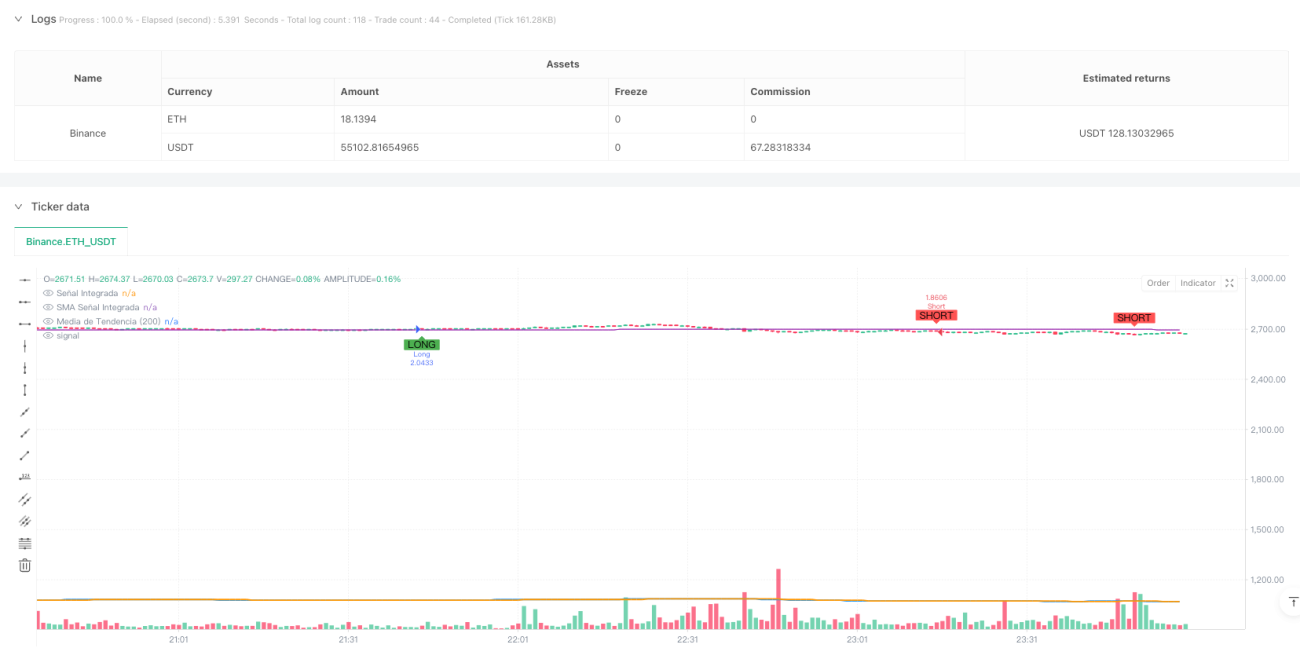
Mã nguồn chiến lược
/*backtest
start: 2025-02-17 00:00:00
end: 2025-02-19 00:00:00
period: 1m
basePeriod: 1m
exchanges: [{"eid":"Binance","currency":"ETH_USDT"}]
*/

//@version=5
strategy("Enhanced Multidimensional Integration Strategy with Nadaraya", overlay=true, initial_capital=10000, currency=currency.USD, default_qty_type=strategy.percent_of_equity, default_qty_value=10)

//────────────────────────────────────────────────────────────────────────────
// 1. Configuration and Weight Optimization Parameters
//────────────────────────────────────────────────────────────────────────────
// Weights can be optimized to favor dimensions with higher historical correlation.
// Base values are maintained but can be fine-tuned.
w_technical   = input.float(0.4,   "Technical Weight",        step=0.05)
w_emotional   = input.float(0.2,   "Emotional Weight",      step=0.05)
w_extrasensor = input.float(0.2,   "Extrasensory Weight", step=0.05)
w_intentional = input.float(0.2,   "Intentional Weight",    step=0.05)

// Parameters for Nadaraya-Watson Smoothing Function:
// Smoothing period and bandwidth affect the "memory" and sensitivity of the signal.
smooth_length = input.int(20, "Smoothing Period", minval=5)
bw_param      = input.float(20, "Bandwidth", minval=1, step=1)

//────────────────────────────────────────────────────────────────────────────
// 2. Risk Management Parameters
//────────────────────────────────────────────────────────────────────────────
// Incorporate stop-loss and take-profit in percentage to protect capital.
// These parameters can be optimized through historical testing.
stopLossPerc   = input.float(1.5, "Stop Loss (%)", step=0.1) / 100   // 1.5% stop-loss
takeProfitPerc = input.float(3.0, "Take Profit (%)", step=0.1) / 100   // 3.0% take-profit

//────────────────────────────────────────────────────────────────────────────
// 3. Additional Filters (Trend and Momentum)
//────────────────────────────────────────────────────────────────────────────
// A long-term moving average is used to confirm the overall trend direction.
trend_length = input.int(200, "Trend MA Period", minval=50)
// RSI is used to confirm momentum. A level of 50 is common to distinguish bullish and bearish phases.
rsi_filter_level = input.int(50, "RSI Confirmation Level", minval=30, maxval=70)

//────────────────────────────────────────────────────────────────────────────
// 4. Definition of Dimensions
//────────────────────────────────────────────────────────────────────────────
tech_series         = close
emotional_series    = ta.rsi(close, 14) / 100
extrasensorial_series = ta.atr(14) / close
intentional_series  = (close - ta.sma(close, 50)) / close

//────────────────────────────────────────────────────────────────────────────
// 5. Nadaraya-Watson Smoothing Function
//────────────────────────────────────────────────────────────────────────────
// This function smooths each dimension using a Gaussian kernel.
// Proper smoothing reduces noise and helps obtain a more robust signal.
nadaraya_smooth(_src, _len, _bw) =>
    if bar_index < _len
        na
    else
        float sumW  = 0.0
        float sumWY = 0.0
        for i = 0 to _len - 1
            weight = math.exp(-0.5 * math.pow(((_len - 1 - i) / _bw), 2))
            sumW  := sumW + weight
            sumWY := sumWY + weight * _src[i]
        sumWY / sumW

//────────────────────────────────────────────────────────────────────────────
// 6. Apply Smoothing to Each Dimension
//────────────────────────────────────────────────────────────────────────────
sm_tech        = nadaraya_smooth(tech_series, smooth_length, bw_param)
sm_emotional   = nadaraya_smooth(emotional_series, smooth_length, bw_param)
sm_extrasens   = nadaraya_smooth(extrasensorial_series, smooth_length, bw_param)
sm_intentional = nadaraya_smooth(intentional_series, smooth_length, bw_param)

//────────────────────────────────────────────────────────────────────────────
// 7. Integration of Dimensions
//────────────────────────────────────────────────────────────────────────────
// The integrated signal is composed of the weighted sum of each smoothed dimension.
// This multidimensional approach seeks to capture different aspects of market behavior.
integrated_signal = (w_technical * sm_tech) + (w_emotional * sm_emotional) + (w_extrasensor * sm_extrasens) + (w_intentional * sm_intentional)
// Additional smoothing of the integrated signal to obtain a reference line.
sma_integrated = ta.sma(integrated_signal, 10)

//────────────────────────────────────────────────────────────────────────────
// 8. Additional Filters to Improve Accuracy and Win Rate
//────────────────────────────────────────────────────────────────────────────
// Trend filter: only trade in the direction of the overall trend, determined by a 200-period SMA.
trendMA = ta.sma(close, trend_length)
// Momentum filter: RSI is used to confirm the strength of the movement (RSI > 50 for long and RSI < 50 for short).
rsi_val = ta.rsi(close, 14)

longFilter  = (close > trendMA) and (rsi_val > rsi_filter_level)
shortFilter = (close < trendMA) and (rsi_val < rsi_filter_level)

// Crossover signals of the integrated signal with its SMA reference.
rawLongSignal  = ta.crossover(integrated_signal, sma_integrated)
rawShortSignal = ta.crossunder(integrated_signal, sma_integrated)
// Incorporate trend and momentum filters to filter false signals.
longSignal  = rawLongSignal and longFilter
shortSignal = rawShortSignal and shortFilter

//────────────────────────────────────────────────────────────────────────────
// 9. Risk Management and Order Generation
//────────────────────────────────────────────────────────────────────────────
// Entries are made based on the filtered integrated signal.
if longSignal
    strategy.entry("Long", strategy.long, comment="Long Entry")
if shortSignal
    strategy.entry("Short", strategy.short, comment="Short Entry")

// Add automatic exits using stop-loss and take-profit to limit losses and secure profits.
// For long positions: stop-loss below entry price and take-profit above.
if strategy.position_size > 0
    strategy.exit("Exit Long", "Long", stop = strategy.position_avg_price * (1 - stopLossPerc), limit = strategy.position_avg_price * (1 + takeProfitPerc))
// For short positions: stop-loss above entry price and take-profit below.
if strategy.position_size < 0
    strategy.exit("Exit Short", "Short", stop = strategy.position_avg_price * (1 + stopLossPerc), limit = strategy.position_avg_price * (1 - takeProfitPerc))

//────────────────────────────────────────────────────────────────────────────
// 10. Visualization on the Chart
//────────────────────────────────────────────────────────────────────────────
plot(integrated_signal, color=color.blue, title="Integrated Signal", linewidth=2)
plot(sma_integrated,      color=color.orange, title="SMA Integrated Signal", linewidth=2)
plot(trendMA,           color=color.purple, title="Trend MA (200)", linewidth=1, style=plot.style_line)
plotshape(longSignal,  title="Long Signal",  location=location.belowbar, color=color.green, style=shape.labelup,   text="LONG")
plotshape(shortSignal, title="Short Signal",  location=location.abovebar, color=color.red,   style=shape.labeldown, text="SHORT")