Chiến lược theo dõi xu hướng giao cắt dải Bollinger nhiều kỳ

Tổng quan
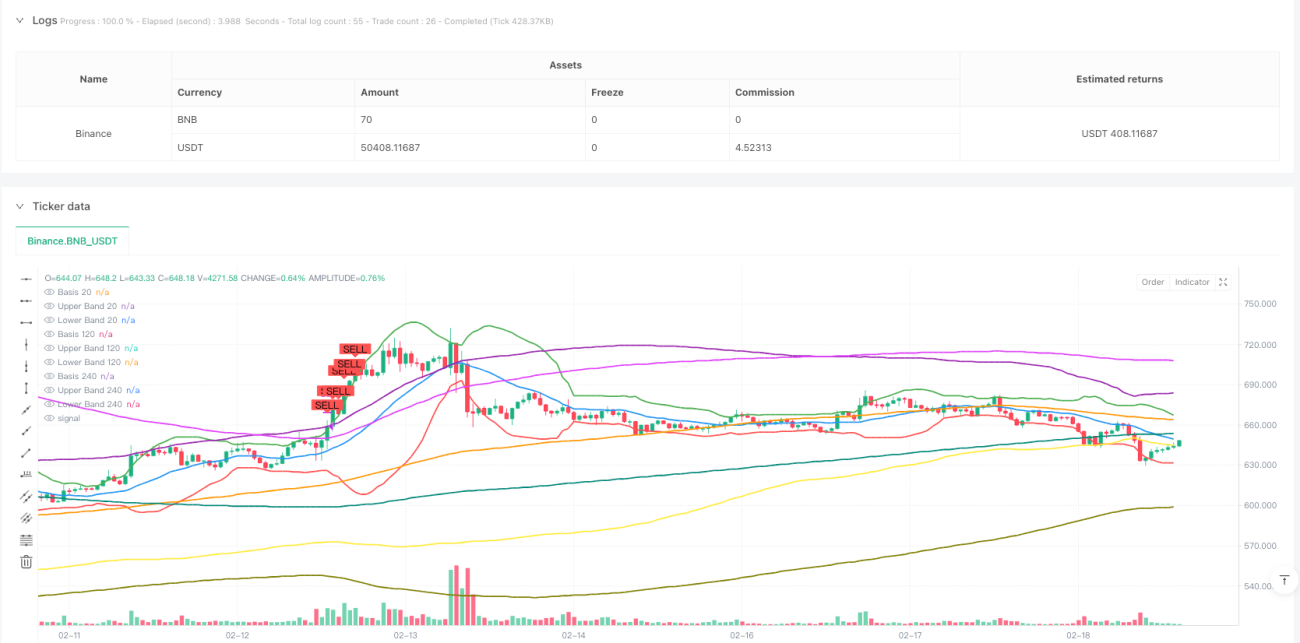
Đây là một chiến lược theo dõi xu hướng dựa trên ba dải Brin. Chiến lược này sử dụng các dải Brin kết hợp với các chu kỳ khác nhau (như: 20, 120 và 240) để nhận biết thị trường đang quá mua và quá bán và tạo ra tín hiệu giao dịch khi giá vượt qua ba dải Brin. Sự kết hợp của các dải Brin đa chu kỳ này có thể lọc hiệu quả các tín hiệu giả và cải thiện độ chính xác của giao dịch.
Nguyên tắc chiến lược
Chiến lược sử dụng ba chu kỳ khác nhau của các vùng Brin ((20 , 120 và 240 chu kỳ), mỗi vùng Brin được tạo thành từ đường trung tâm ((SMA) và đường đi lên xuống ((2 lần chênh lệch tiêu chuẩn). Khi giá đồng thời phá vỡ đường đi xuống của ba vùng Brin, cho thấy thị trường có thể bị bán tháo, hệ thống phát ra nhiều tín hiệu; khi giá đồng thời phá vỡ đường đi lên của ba vùng Brin, cho thấy thị trường có thể bị mua quá mức, hệ thống phát ra tín hiệu giá bằng bằng cách quan sát các vùng Brin trong nhiều chu kỳ, bạn có thể xác định tốt hơn sức mạnh và tính bền vững của xu hướng thị trường.
Lợi thế chiến lược
- Cơ chế xác nhận nhiều lần: Sử dụng ba chu kỳ khác nhau của băng Brin làm bộ lọc, có thể giảm hiệu quả tín hiệu giả.
- Khả năng theo dõi xu hướng: Chiến lược có thể thích ứng với các môi trường thị trường khác nhau thông qua tính năng điều chỉnh động của Brinband.
- Kiểm soát rủi ro rõ ràng: Brinh tự nó có ý nghĩa thống kê, cung cấp một vị trí tham chiếu rõ ràng cho nhập cảnh và xuất cảnh.
- Thể điều chỉnh tham số: Chiến lược cung cấp các thiết lập tham số của chu kỳ và nhân của Brin, có thể được tối ưu hóa theo các đặc điểm thị trường khác nhau.
Rủi ro chiến lược
- Rủi ro thị trường ngang: có thể tạo ra các tín hiệu sai lệch thường xuyên trong thị trường biến động, dẫn đến giao dịch quá mức.
- Rủi ro bị tụt hậu: Có thể bỏ lỡ thời gian đầu vào tốt nhất tại điểm chuyển hướng vì sử dụng trung bình di chuyển có chu kỳ dài hơn.
- Rủi ro quản lý tài chính: Nếu không thiết lập vị trí dừng lỗ thích hợp, có thể chịu tổn thất lớn khi biến động mạnh.
- Tùy thuộc tham số: Các tham số tối ưu có thể có sự khác biệt lớn trong các môi trường thị trường khác nhau và cần được tối ưu hóa thường xuyên.
Hướng tối ưu hóa chiến lược
- Tiếp theo, có thể thêm khối lượng giao dịch như một chỉ số phụ trợ để cải thiện độ tin cậy của tín hiệu.
- Tối ưu hóa cơ chế dừng lỗ: khuyến nghị thêm dừng theo dõi hoặc dừng ATR để kiểm soát rủi ro tốt hơn.
- Thêm chỉ số xác nhận xu hướng: có thể được kiểm tra chéo với các chỉ số xu hướng khác (như MACD, DMI, v.v.).
- Điều chỉnh tham số động: Các tham số của Brin Belt có thể được điều chỉnh tự động theo biến động của thị trường, giúp cải thiện khả năng thích ứng của chiến lược.
- Cải thiện bộ lọc tín hiệu: Bạn có thể thêm các điều kiện như bộ lọc thời gian giao dịch, bộ lọc tỷ lệ dao động để giảm tín hiệu giả.
Tóm tắt
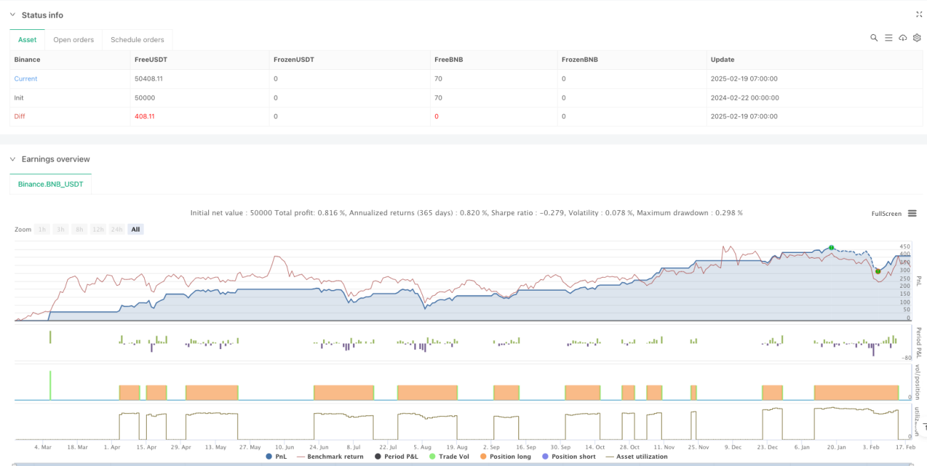
Đây là một chiến lược theo dõi xu hướng dựa trên nhiều chu kỳ của Brin, xác nhận tín hiệu giao dịch thông qua giao thoa của ba Brin, có độ tin cậy và khả năng thích ứng cao. Ưu điểm cốt lõi của chiến lược là cơ chế xác nhận nhiều lần và hệ thống kiểm soát rủi ro rõ ràng, nhưng cũng cần chú ý đến vấn đề hiệu suất và tối ưu hóa tham số trong thị trường xung đột.
- 1