
Tổng quan
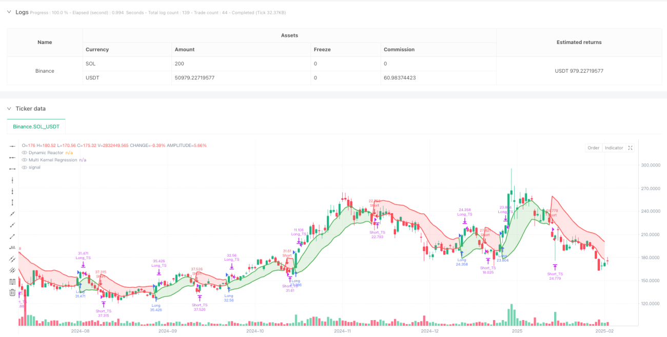
Chiến lược này là một hệ thống theo dõi xu hướng kết hợp Dynamic Reactor và Multi-Kernel Regression. Nó nắm bắt xu hướng thị trường bằng cách kết hợp kênh ATR, đường SMA và Gaussian Nuclear Regression với Epanechnikov Nuclear Regression và lọc tín hiệu bằng chỉ số RSI. Chiến lược này cũng bao gồm một hệ thống quản lý vị thế hoàn chỉnh, bao gồm các tính năng như dừng lỗ động, mục tiêu lợi nhuận nhiều lần và theo dõi dừng lỗ.
Nguyên tắc chiến lược
Cốt lõi của chiến lược bao gồm hai phần chính. Phần đầu tiên là bộ phản ứng động (DR), nó xây dựng một kênh giá tự điều chỉnh dựa trên ATR và SMA. Độ rộng của kênh được xác định bởi số ATR và vị trí của kênh được điều chỉnh theo sự di chuyển của SMA.
Lợi thế chiến lược
- Khả năng thích ứng: Bằng cách kết hợp các phản ứng viên động và hồi quy đa lõi, chiến lược có thể tự động thích ứng với các môi trường thị trường và điều kiện biến động khác nhau.
- Quản lý rủi ro tốt: bao gồm nhiều cơ chế kiểm soát rủi ro như dừng động, thu lợi nhuận theo đợt và theo dõi dừng lỗ.
- Chất lượng tín hiệu cao: có thể giảm hiệu quả tín hiệu giả thông qua lọc RSI và xác nhận chéo của hai đường.
- Hiệu quả tính toán cao: Mặc dù sử dụng thuật toán hồi quy lõi phức tạp, nhưng đảm bảo hiệu suất thực tế của chiến lược bằng cách tối ưu hóa phương pháp tính toán.
Rủi ro chiến lược
- Tính nhạy cảm của tham số: hiệu quả của chiến lược phụ thuộc rất nhiều vào các thiết lập tham số như ATR, băng thông hàm lõi và các tham số không đúng có thể dẫn đến giao dịch quá mức hoặc bỏ lỡ cơ hội.
- Sự chậm trễ: Do sử dụng thuật toán trung bình di chuyển và hồi quy, có thể có một số chậm trễ trong giao dịch nhanh.
- Thị trường thích ứng: Chiến lược này hoạt động tốt trong thị trường xu hướng, nhưng có thể thường xuyên tạo ra tín hiệu sai trong thị trường chấn động.
- Tính phức tạp của tính toán: tính toán phần hồi quy đa lõi là phức tạp hơn, cần chú ý đến tối ưu hóa hiệu suất trong môi trường giao dịch tần số cao.
Hướng tối ưu hóa chiến lược
- Các tham số tự thích ứng: có thể giới thiệu cơ chế thích ứng, điều chỉnh động số nhân ATR và băng thông hàm lõi theo biến động của thị trường.
- Tối ưu hóa tín hiệu: Xem xét thêm các chỉ số phụ trợ như khối lượng giao dịch, hình thức giá để tăng độ tin cậy của tín hiệu.
- Kiểm soát rủi ro: tỷ lệ giữa mục tiêu dừng lỗ và mục tiêu thu lợi nhuận có thể được điều chỉnh theo biến động của thị trường.
- Thị trường lọc: thêm mô-đun nhận diện môi trường thị trường, sử dụng chiến lược giao dịch khác nhau trong các điều kiện thị trường khác nhau.
Tóm tắt
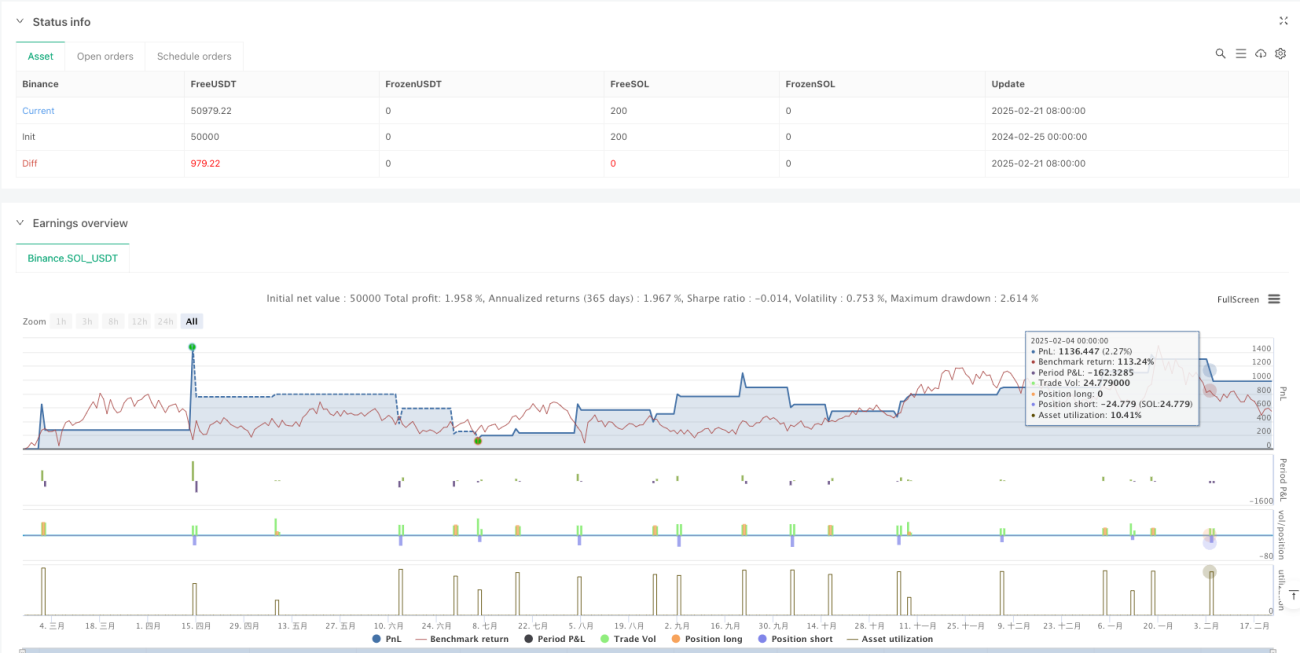
Đây là một hệ thống giao dịch hoàn chỉnh kết hợp các phương pháp thống kê hiện đại và phân tích kỹ thuật truyền thống. Chiến lược này cho thấy khả năng thích ứng và ổn định tốt thông qua sự kết hợp sáng tạo của phản ứng viên động và hồi quy đa lõi, cùng với cơ chế quản lý rủi ro tốt. Mặc dù có một số nơi cần được tối ưu hóa, chiến lược này có khả năng duy trì hiệu suất ổn định trong các môi trường thị trường khác nhau thông qua cải tiến liên tục và tối ưu hóa tham số.
/*backtest
start: 2024-07-20 00:00:00
end: 2025-07-19 08:00:00
period: 1d
basePeriod: 1d
exchanges: [{"eid":"Binance","currency":"ETH_USDT","balance":2000000}]
*/

//@version=5
strategy("DR+MKR Signals – Band SL, Multiple TP & Trailing Stop", overlay=true, default_qty_value=10)

// =====================================================================- 1