Chiến lược giao dịch theo xu hướng động hồi quy đa lõi

DR MKR ATR SMA MA200 TP SL
Ngày tạo: 2025-02-24 09:27:50 sửa đổi lần cuối: 2025-02-24 09:27:50
sao chép: 0 Số nhấp chuột: 805
2
tập trung vào
319
Người theo dõi

Chiến lược giao dịch theo xu hướng động hồi quy đa lõi Chiến lược giao dịch theo xu hướng động hồi quy đa lõi

Tổng quan

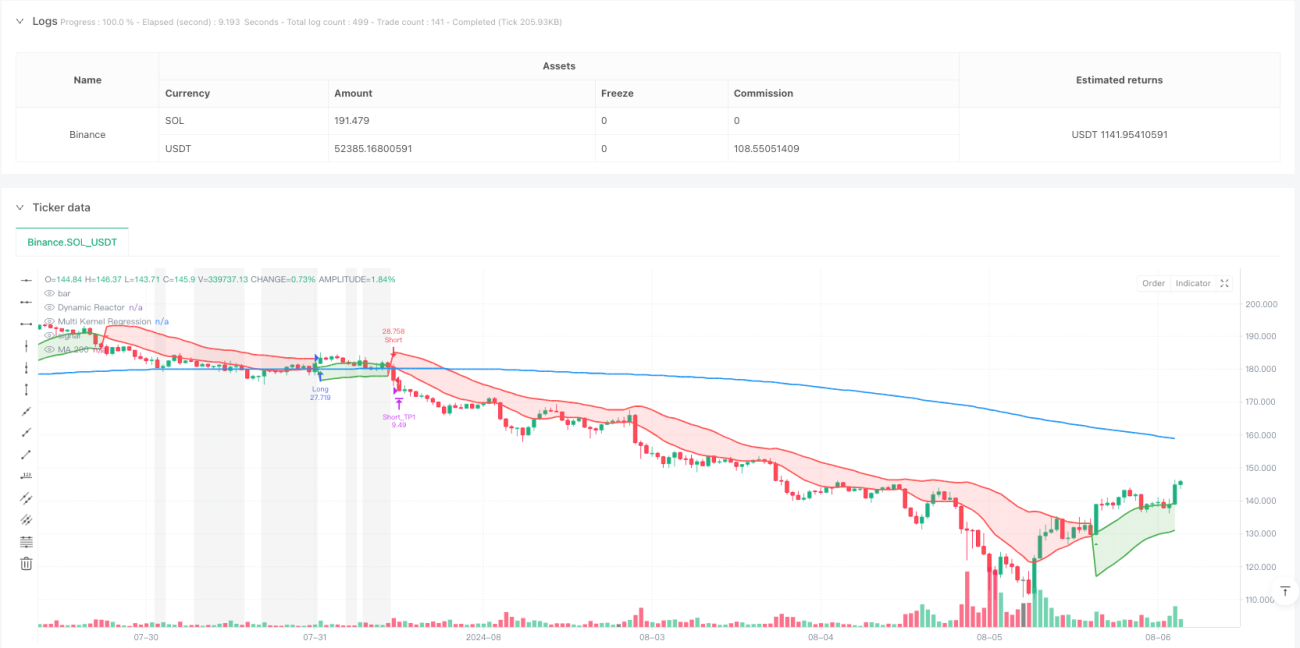
Đây là một chiến lược giao dịch theo dõi xu hướng kết hợp phản ứng động và hồi quy đa hạt nhân. Chiến lược này tính toán đường hỗ trợ / kháng động thông qua ATR và SMA, và sử dụng sự trở lại kết hợp của hạt nhân Gauss và hạt nhân Epanechnikov để xác định xu hướng thị trường.

Nguyên tắc chiến lược

Chiến lược bao gồm bốn phần cốt lõi:

  1. Phản ứng xu hướng động ((DR): Sử dụng ATR và SMA để xây dựng các vùng hỗ trợ / kháng cự động, định hướng xu hướng dựa trên vị trí giá. Sử dụng vùng dưới làm hỗ trợ trong xu hướng tăng và vùng trên làm kháng cự trong xu hướng giảm.

  2. Multi-Core Regression (MKR): Phản hồi giá kết hợp với lõi Gaussian và lõi Epanechnikov để thực hiện sự kết hợp tối ưu của hai hàm lõi thông qua các tham số trọng lượng có thể điều chỉnh. Phương pháp này có thể nắm bắt tốt hơn các đặc điểm động của biến động giá.

  3. Bộ lọc xu hướng MA200: Sử dụng đường trung bình 200 ngày làm chỉ số xu hướng dài hạn, chỉ cho phép giao dịch khi giá có xu hướng rõ ràng với MA200 và xác định thời gian sắp xếp bằng tham số ConsolidationRange.

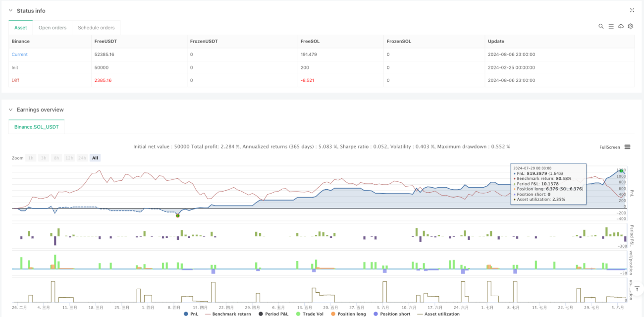
  4. Hệ thống quản lý tiền: Sử dụng mục tiêu lợi nhuận ba lần ((1,5%, 3,0%, 4,5%) và 1% dừng lỗ, phân bổ vị trí theo tỷ lệ 33% -33% -34%, đồng thời kiểm soát rủi ro để tối đa hóa lợi nhuận.

Lợi thế chiến lược

  1. Độ tin cậy của nhận dạng xu hướng: tăng độ chính xác của phán đoán xu hướng thông qua xác nhận kép của DR và MKR.
  2. Tính toàn vẹn của quản lý rủi ro: sử dụng kết hợp lợi nhuận phân đoạn và dừng lỗ thống nhất, bảo vệ lợi nhuận và hạn chế tổn thất.
  3. Khả năng thích ứng: Phương pháp hồi quy đa lõi thích ứng tốt hơn với các điều kiện thị trường khác nhau.
  4. Các tín hiệu giao dịch rõ ràng: điểm chuyển hướng có chỉ dẫn đồ họa rõ ràng.
  5. Cơ chế lọc được cải thiện: Xác định và loại bỏ môi trường thị trường bất lợi thông qua MA200 và kỳ thu xếp.

Rủi ro chiến lược

  1. Rủi ro tối ưu hóa tham số: Tối ưu hóa quá mức có thể dẫn đến quá phù hợp, làm giảm hiệu suất thực tế của chiến lược.
  2. Rủi ro bị tụt hậu: cả đường trung bình và chỉ số hồi phục đều có một số độ tụt hậu, có thể bỏ lỡ các bước ngoặt quan trọng.
  3. Tùy thuộc vào môi trường thị trường: có thể không hoạt động tốt trong thị trường biến động mạnh hoặc thị trường ngang.
  4. Rủi ro thực hiện: Nhiều lệnh dừng lỗ có thể không được thực hiện đầy đủ do vấn đề về thanh khoản.

Hướng tối ưu hóa chiến lược

  1. Điều chỉnh tham số động: có thể tự động điều chỉnh ATR nhân và chu kỳ trở lại theo biến động của thị trường.
  2. Tăng cường tín hiệu xác nhận: có thể thêm các chỉ số phụ trợ như số lượng giao thông, tỷ lệ dao động để tăng độ tin cậy tín hiệu.
  3. Tối ưu hóa quản lý vị thế: có thể thực hiện quản lý vị thế động dựa trên biến động.
  4. Phân loại môi trường thị trường: thêm mô-đun nhận dạng trạng thái thị trường, sử dụng các thiết lập tham số khác nhau trong các môi trường thị trường khác nhau.

Tóm tắt

Chiến lược này xây dựng một hệ thống giao dịch hoàn chỉnh bằng cách kết hợp nhiều chỉ số kỹ thuật và các phương pháp thống kê tiên tiến. Ưu điểm của chiến lược là nắm bắt chính xác xu hướng và hệ thống quản lý rủi ro tốt, nhưng cũng cần chú ý đến các vấn đề tối ưu hóa tham số và khả năng thích ứng của thị trường.

Mã nguồn chiến lược
/*backtest
start: 2024-02-25 00:00:00
end: 2024-08-07 00:00:00
period: 1h
basePeriod: 1h
exchanges: [{"eid":"Binance","currency":"SOL_USDT"}]
*/

//@version=5
strategy("DR + Multi Kernel Regression + Signals + MA200 with TP/SL (Optimized)", overlay=true, shorttitle="DR+MKR+Signals+MA200_TP_SL_Opt", pyramiding=0, default_qty_type=strategy.percent_of_equity, default_qty_value=10)

// =====================================================================
// PARTEA 1: Dynamic Reactor – linie unică colorată în funcție de trend
// =====================================================================
// Parametri pentru Dynamic Reactor
atrLength  = input.int(14, title="Lungimea ATR", minval=1)
smaLength  = input.int(20, title="Lungimea SMA", minval=1)
multiplier = input.float(1.5, title="Multiplicator ATR", minval=0.1, step=0.1)
// Calculăm ATR și SMA
atrValue = ta.atr(atrLength)
smaValue = ta.sma(close, smaLength)
// Benzile de bază
basicUpper = smaValue + atrValue * multiplier
basicLower = smaValue - atrValue * multiplier
// Calculăm benzile finale (similar cu SuperTrend)
var float finalUpper = basicUpper
var float finalLower = basicLower
if bar_index > 0
    finalUpper := close[1] > finalUpper[1] ? math.max(basicUpper, finalUpper[1]) : basicUpper
    finalLower := close[1] < finalLower[1] ? math.min(basicLower, finalLower[1]) : basicLower
// Determinăm trendul curent:
// - Dacă prețul curent este peste finalUpper din bara anterioară → uptrend (1)
// - Dacă prețul este sub finalLower din bara anterioară → downtrend (-1)
// - Altfel, păstrăm trendul precedent.
var int trend = 1
if bar_index > 0
    trend := close > finalUpper[1] ? 1 : close < finalLower[1] ? -1 : nz(trend[1], 1)
// Linia Dynamic Reactor:
// - În uptrend se utilizează finalLower (nivel de suport)
// - În downtrend se utilizează finalUpper (nivel de rezistență)
drLine = trend == 1 ? finalLower : finalUpper
// Plotăm linia Dynamic Reactor
p_dr = plot(drLine, color=trend == 1 ? color.green : color.red, title="Dynamic Reactor", linewidth=2)


// =====================================================================
// PARTEA 2: Multi Kernel Regression
// =====================================================================
// Parametri pentru regresia cu kernel
regLength = input.int(50, title="Perioada regresiei", minval=1)
h1        = input.float(10.0, title="Bandă Gaussiană (h1)", minval=0.1)
h2        = input.float(10.0, title="Bandă Epanechnikov (h2)", minval=0.1)
alpha     = input.float(0.5, title="Pondere Kernel Gaussian (0-1)", minval=0, maxval=1)
// Funcție: regresie cu kernel Gaussian
f_gaussian_regression(bw) =>
    num = 0.0
    den = 0.0
    for i = 0 to regLength - 1
        // Kernel Gaussian: K(x) = exp(-0.5 * (i/bw)^2)
        weight = math.exp(-0.5 * math.pow(i / bw, 2))
        num += close[i] * weight
        den += weight
    num / (den == 0 ? 1 : den)
// Funcție: regresie cu kernel Epanechnikov
f_epanechnikov_regression(bw) =>
    num = 0.0
    den = 0.0
    for i = 0 to regLength - 1
        ratio = i / bw
        // Kernel Epanechnikov: K(u) = 1 - u^2 pentru |u| <= 1, altfel 0
        weight = math.abs(ratio) <= 1 ? (1 - math.pow(ratio, 2)) : 0
        num += close[i] * weight
        den += weight
    num / (den == 0 ? 1 : den)
// Calculăm regresiile pentru fiecare kernel
regGauss = f_gaussian_regression(h1)
regEpan  = f_epanechnikov_regression(h2)
// Combinăm rezultatele celor două regresii
multiKernelRegression = alpha * regGauss + (1 - alpha) * regEpan
// Plotăm linia Multi Kernel Regression
p_mkr = plot(multiKernelRegression, color=trend == 1 ? color.green : color.red, title="Multi Kernel Regression", linewidth=2)

// Adăugăm ceata (fill) între Dynamic Reactor și Multi Kernel Regression
fillColor = trend == 1 ? color.new(color.green, 80) : color.new(color.red, 80)
fill(p_dr, p_mkr, color=fillColor, title="Trend Fill")


// =====================================================================
// PARTEA 2.1: MA 200 și evidențierea consolidării
// =====================================================================
// Calculăm MA 200 pentru trend pe termen lung
ma200 = ta.sma(close, 200)
p_ma200 = plot(ma200, color=color.blue, title="MA 200", linewidth=2)
// Parametru pentru detectarea consolidării (cât de aproape trebuie să fie prețul de MA200, în %)
consolidationRange = input.float(1.0, title="Consolidation Range (%)", minval=0.1, step=0.1)
// Determinăm dacă suntem într-o fază de consolidare (prețul este în interiorul unui interval mic în jurul MA200)
isConsolidation = (math.abs(close - ma200) / ma200 * 100) < consolidationRange
// Colorăm fundalul graficului cu un gri translucid atunci când e consolidare
bgcolor(isConsolidation ? color.new(color.gray, 90) : na, title="Consolidation BG")


// =====================================================================
// PARTEA 3: Semnale Buy și Sell
// =====================================================================
// Semnale de intrare:
// - Buy Signal: când linia Multi Kernel Regression trece peste linia Dynamic Reactor
// - Sell Signal: când linia Multi Kernel Regression trece sub linia Dynamic Reactor
buySignal  = ta.crossover(multiKernelRegression, drLine)
sellSignal = ta.crossunder(multiKernelRegression, drLine)

// Plotăm semnalele pe grafic
plotshape(buySignal, style=shape.triangleup, location=location.belowbar, color=color.green, size=size.tiny, title="Buy Signal")
plotshape(sellSignal, style=shape.triangledown, location=location.abovebar, color=color.red, size=size.tiny, title="Sell Signal")

// Setăm condiții de alertă
alertcondition(buySignal, title="Buy Alert", message="Buy Signal: Kernel is above Dynamic Reactor")
alertcondition(sellSignal, title="Sell Alert", message="Sell Signal: Kernel is below Dynamic Reactor")


// =====================================================================
// PARTEA 4: Trade Management – Intrări, 3 TP și 1 SL
// =====================================================================
// Parametrii pentru TP și SL (valori ajustate pentru un raport risc-recompensă mai favorabil)
tp1Perc = input.float(1.5, title="TP1 (%)", minval=0.1, step=0.1)
tp2Perc = input.float(3.0, title="TP2 (%)", minval=0.1, step=0.1)
tp3Perc = input.float(4.5, title="TP3 (%)", minval=0.1, step=0.1)
slPerc  = input.float(1.0, title="Stop Loss (%)", minval=0.1, step=0.1)

// ---- Intrări de tranzacționare cu filtrare suplimentară pe baza trendului MA200 și consolidării ----
// Pentru poziții long, intrăm doar când prețul este peste MA200 și nu este în consolidare.
// Pentru poziții short, intrăm doar când prețul este sub MA200 și nu este în consolidare.
if (buySignal and close > ma200 and not isConsolidation)
    strategy.entry("Long", strategy.long)

if (sellSignal and close < ma200 and not isConsolidation)
    strategy.entry("Short", strategy.short)

// ---- Gestionarea ordinelor pentru poziții long ----
if (strategy.position_size > 0)
    entryPrice = strategy.position_avg_price
    // Calculăm nivelurile de TP și SL pentru poziția long
    long_sl = entryPrice * (1 - slPerc / 100)
    long_tp1 = entryPrice * (1 + tp1Perc / 100)
    long_tp2 = entryPrice * (1 + tp2Perc / 100)
    long_tp3 = entryPrice * (1 + tp3Perc / 100)
    
    // Plasăm TP-urile (alocări: 33%, 33% și 34%)
    strategy.exit("Long_TP1", from_entry="Long", limit=long_tp1, qty_percent=33, comment="TP1")
    strategy.exit("Long_TP2", from_entry="Long", limit=long_tp2, qty_percent=33, comment="TP2")
    strategy.exit("Long_TP3", from_entry="Long", limit=long_tp3, qty_percent=34, comment="TP3")
    
    // Plasăm ordinul de SL pentru poziția long
    strategy.exit("Long_SL", from_entry="Long", stop=long_sl, comment="SL")

// ---- Gestionarea ordinelor pentru poziții short ----
if (strategy.position_size < 0)
    entryPrice = strategy.position_avg_price
    // Calculăm nivelurile de TP și SL pentru poziția short
    short_sl = entryPrice * (1 + slPerc / 100)
    short_tp1 = entryPrice * (1 - tp1Perc / 100)
    short_tp2 = entryPrice * (1 - tp2Perc / 100)
    short_tp3 = entryPrice * (1 - tp3Perc / 100)
    
    // Plasăm TP-urile (alocări: 33%, 33% și 34%)
    strategy.exit("Short_TP1", from_entry="Short", limit=short_tp1, qty_percent=33, comment="TP1")
    strategy.exit("Short_TP2", from_entry="Short", limit=short_tp2, qty_percent=33, comment="TP2")
    strategy.exit("Short_TP3", from_entry="Short", limit=short_tp3, qty_percent=34, comment="TP3")
    
    // Plasăm ordinul de SL pentru poziția short
    strategy.exit("Short_SL", from_entry="Short", stop=short_sl, comment="SL")