Tổng quan

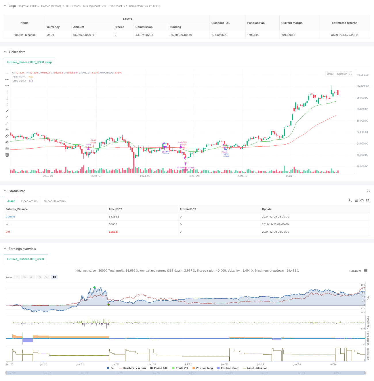
Chiến lược này là một hệ thống theo dõi xu hướng kết hợp các chỉ số động trung bình của chỉ số biến thể (VIDYA) với các dải Bollinger (Bollinger Bands) và tích hợp các cơ chế dừng nhiều tầng. Không giống như các chiến lược xu hướng truyền thống, hệ thống này sử dụng một cách thu lợi nhuận thích ứng hơn để phân biệt các vị trí trống nhiều hơn thông qua chỉ số ATR và mục tiêu phần trăm độc đáo.

Nguyên tắc chiến lược

Cốt lõi của chiến lược là sử dụng hai chỉ số VIDYA nhanh và chậm để phân tích xu hướng giá cả, đồng thời xem xét sự biến động của thị trường. Công thức tính toán của chỉ số VIDYA là:
Tỷ lệ phẳng của α = 2/α + 1
VIDYA (t) = α * k * giá (t) + (1 - α * k) * VIDYA (t-1)
Trong đó k = <unk> chán động cơ dao động (MO) 100

Brinband làm bộ lọc tỷ lệ dao động:
Đường lên = MA + (K * chênh lệch chuẩn)
Đường sắt dưới = MA - (K * chênh lệch tiêu chuẩn)

Điều kiện tham gia:

• Nhiều đầu: Giá phá vỡ VIDYA chậm và VIDYA nhanh xu hướng lên, đồng thời giá phá vỡ dây chuyền Brin trên đường ray
• Blank: Giá giảm xuống thấp hơn VIDYA chậm và VIDYA nhanh xu hướng giảm, đồng thời giá giảm xuống thấp hơn Brin

Các hệ thống ngăn chặn đa tầng bao gồm:

1. Dừng dựa trên ATR
2. Cụm dựa trên tỷ lệ phần trăm
3. Giao dịch không đầu tư sử dụng nhân để tăng tỷ lệ dừng

Lợi thế chiến lược

1. Tính linh hoạt: Chỉ số Vidia có thể tự động điều chỉnh theo biến động của thị trường, nhạy cảm hơn so với đường trung bình truyền thống
2. Quản lý rủi ro tốt: Hệ thống ngăn chặn nhiều lớp có thể khóa lợi nhuận ở các mức giá khác nhau
3. Phân biệt xử lý: sử dụng chiến lược chặn khác nhau đối với các vị trí trống, phù hợp hơn với đặc điểm của thị trường
4. Bộ lọc tỷ lệ dao động: Brinband được sử dụng để lọc các tín hiệu đột phá giả
5. Tính linh hoạt: có thể điều chỉnh các tham số theo các điều kiện thị trường khác nhau

Rủi ro chiến lược

1. Rủi ro thị trường chấn động: Có thể tạo ra tín hiệu sai lệch trên thị trường ngang
2. Tác động điểm trượt: Nhiều điểm dừng có thể dẫn đến sai lệch giá thực hiện do điểm trượt
3. Tùy thuộc tham số: Các tham số có thể cần được điều chỉnh thường xuyên trong các môi trường thị trường khác nhau
4. Sự phức tạp của hệ thống: nhiều lớp ngăn chặn làm tăng sự phức tạp của chiến lược
5. Căng thẳng quản lý tài chính: Nhiều lệnh ngừng hoạt động có thể làm tăng khó khăn trong việc quản lý vị trí

Hướng tối ưu hóa chiến lược

1. Điều chỉnh tham số động: Có thể phát triển hệ thống tham số thích ứng, tự động điều chỉnh theo điều kiện thị trường
2. Nhận biết môi trường thị trường: thêm mô-đun phán đoán môi trường thị trường, sử dụng các tham số khác nhau trong các điều kiện thị trường khác nhau
3. Tối ưu hóa dừng lỗ: tăng cơ chế dừng lỗ động và tăng khả năng kiểm soát rủi ro
4. Bộ lọc tín hiệu: Tăng số lượng giao thông và các chỉ số phụ trợ để tăng độ tin cậy tín hiệu
5. Quản lý vị trí: Phát triển thuật toán phân bổ vị trí thông minh hơn

Tóm tắt

Chiến lược này tạo ra một hệ thống theo dõi xu hướng toàn diện bằng cách kết hợp tính thích ứng động của chỉ số VIDYA và chức năng lọc tỷ lệ biến động của Brin Belt. Cơ chế chặn nhiều lớp và phương pháp xử lý đa không gian khác biệt, giúp nó có khả năng lợi nhuận và kiểm soát rủi ro tốt. Tuy nhiên, người dùng cần chú ý đến sự thay đổi của môi trường thị trường, điều chỉnh tham số khi thích hợp và xây dựng một hệ thống quản lý tài chính tốt.