Multi-indicator Strategy to Identify Trading Inflection Points in Quant Trading

Author: ChaoZhang, Date: 2023-11-02 14:09:34
Tags:

Overview

This strategy integrates 5 major indicators including EMA, VWAP, MACD, Bollinger Bands and Schaff Trend Cycle to identify inflection points where price reverses within a certain range, and generates buy and sell signals. The advantage of this strategy is the flexibility to combine different indicators based on varying market conditions to reduce false signals and improve profitability. However, there are also risks of lagging signal identification and improper parameter tuning. Overall, the strategy has a clear logic flow and strong practical value.

Strategy Logic

EMA judges overall trend direction, only buy with trend
VWAP judges institutional money flow, only buy when institutions are buying
MACD judges short-term trend and momentum change, MACD line crossover signal line is buy/sell signal
Bollinger Bands judge overbought and oversold conditions, price breaking out of bands suggests buy/sell signals
Schaff Trend Cycle judges short-term range-bound structure, exceeding high/low thresholds suggests buy/sell signals
Send buy/sell orders when all 5 indicators agree on the signal
Set stop loss and take profit to optimize capital management

Advantages

Lower false signals with multi-indicator combo

Using a combination of indicators like EMA, VWAP, MACD, BB and STC allows cross-validation to weed out false signals from any individual indicators, improving reliability.

Customizable indicators

Ability to turn on/off indicators allows combining ideal indicators for different products and market environments, improving adaptability.

Optimized capital management

Stop loss and take profit allows limiting single trade loss and locking in profits, enabling better capital management.

Clear strategy logic

Simple intuitive indicators used with detailed code comments make the overall strategy logic easy to understand and modify.

Strong practicality

Widely used indicators with reasonable tuning allows live trading with decent results right away without extensive optimizations.

Risks

Lagging signal identification risk

EMA, MACD etc have lag in identifying price changes, which may cause missing best entry timing.

Improper parameter tuning risk

Bad indicator parameters will generate excessive false signals and break strategy.

No guarantee of win rate

Multi-indicator combo improves but does not guarantee win rate. Market regime change can cause win rate decline.

Stop loss set too tight

If stop loss is too tight, normal price fluctuations may get stopped out causing unnecessary losses.

Enhancement Opportunities

Add ML model for signal reliability scoring

Train model to score multi-indicator signals on reliability, filter out false signals.

Add momentum indicators for accumulation identification

Add quant indicators like OBV to identify price accumulation, improving buy point certainty.

Optimize stop loss and take profit logic

Research more suitable trailing stop or profit taking logic for this strategy to better optimize capital management.

Parameter optimization

Conduct more systematic backtests to find optimal parameters for each indicator, improving robustness.

Add auto trading

Connect to trading API to allow auto order execution, enabling fully automated hands-off strategy execution.

Conclusion

This strategy combines strengths of multiple technical indicators with a clear logic flow and strong practical value. It can serve as discretionary trading decision support or direct algorithmic trading. But optimization and tuning based on specific product and market environment is needed to reduce risk and improve stability before consistent profitable live trading.

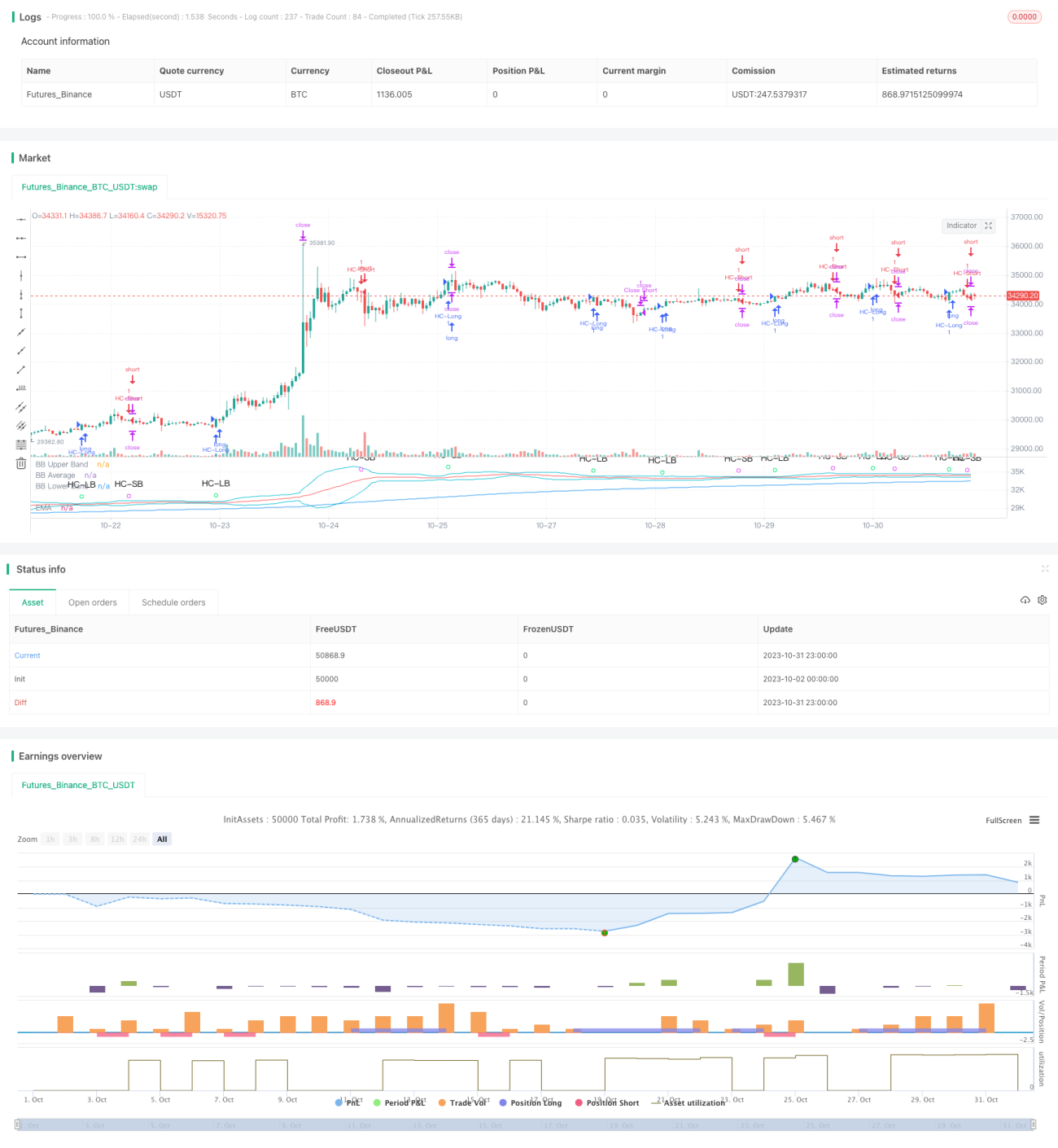
/*backtest
start: 2023-10-02 00:00:00
end: 2023-11-01 00:00:00
period: 1h
basePeriod: 15m
exchanges: [{"eid":"Futures_Binance","currency":"BTC_USDT"}]
*/

//@version=4

// This source code is subject to the terms of the Mozilla Public License 2.0 at https://mozilla.org/MPL/2.0/
// © MakeMoneyCoESTB2020

//*********************Notes for continued work***************
//3) add a Table of contents to each section of code
//4) add candle stick pattern considerations to chart
//5) add an input value for DTE range to backtest
//7) add abilit to turn on/off MACD plot
//9)
//************************************************************


//Hello my fellow investors
//After hours of reading, backtesting, and YouTube video watching
//I discovered that 200EMA, VWAP, BB, MACD, and STC 
//produce the most consistent results for investment planning.
//This strategy allows you to pick between the aforementioned indicators or layer them together.
//It works on the pricipal of:
//1) Always follow the market trend - buy/sell above/below 200EMA
//2) Follow corporate investing trends - buy/sell above/below VWAP
//3) Apply MACD check - buy--> MACD line above signal line 
// and corssover below histogram \\ sell --> MACD line below signal line 
// and crossover above histogram.
//4) Check volitility with price against BB limits upper/Sell or lower/buy
//5) When STC crosses about 10 buy and when it drops below 90 sell
//6) Exit position when stop loss is triggered or profit target is hit.  BB also provides a parameter to exit positions.

//This code is the product of many hours of hard work on the part of the greater tradingview community.  The credit goes to everyone in the community who has put code out there for the greater good.

//Happy Hunting!



//Title
// strategy("WOMBO COMBO: 100/200EMA & VWAP & MACD", shorttitle="WOMBO COMBO", default_qty_type=strategy.percent_of_equity, default_qty_value=1.5, initial_capital=10000,slippage=2, currency=currency.USD, overlay=true)

//define calculations price source
price = input(title="Price Source", defval=close)


//***************************
//Calculate 20/50/100/200EMA 
EMAlength = input(title="EMA_Length", defval=200)
EMA=ema(price, EMAlength)
//plot EMA
ColorEMA=EMAlength==200?color.blue:EMAlength==100?color.aqua:EMAlength==50?color.orange:color.red
plot(EMA, title = "EMA", color = ColorEMA)


//*****************************
//calculate VWAP
ColorVWAP = (price > vwap) ? color.lime : color.maroon
plot(vwap, title = "VWAP", color=ColorVWAP, linewidth=2)


//*****************************
//calculate MACD
//define variables for speed
fast = 12, slow = 26
//define parameters to calculate MACD
fastMA = ema(price, fast)
slowMA = ema(price, slow)
//define MACD line
macd = fastMA - slowMA
//define SIGNAL line
signal = sma(macd, 9)
//plot MACD line
//plot(macd, title = "MACD",  color=color.orange)
//plot signal line
//plot(signal, title = "Signal", color=color.purple)
//plot histogram
//define histogram colors
//col_grow_above = color.green
//col_grow_below = color.red
//col_fall_above = color.lime
//col_fall_below = color.maroon
//define histogram value
//hist = macd - signal
//plot histogram
//plot(hist, title="Histogram", style=plot.style_columns, color=(hist>=0 ? (hist[1] < hist ? col_grow_above : col_fall_above) : (hist[1] < hist ? col_grow_below : col_fall_below) ), transp=0 )


//***************************************
//Calculate Bollinger Bands
//Define BB input variables
//lengthBB = input(20, minval=1)
//multBB = input(2.0, minval=0.001, maxval=50)
lengthBB = 20
multBB = 2
//define BB average
basisBB = sma(price, lengthBB)
//define BB standar deviation
devBB = multBB * stdev(price, lengthBB)
//define BB upper and lower limits
upperBB = basisBB + devBB
lowerBB = basisBB - devBB
//Plot BB graph
ShowBB = input(title="Show BB", defval="Y", type=input.string, options=["Y", "N"])
transP = (ShowBB=="Y") ? 0 : 100
plot (upperBB, title = "BB Upper Band", color = color.aqua, transp=transP)
plot (basisBB, title = "BB Average", color = color.red, transp=transP)
plot (lowerBB, title = "BB Lower Band", color = color.aqua, transp=transP)


//*************************************************
//Calculate STC
//fastLength = input(title="MACD Fast Length", type=input.integer, defval=12)
//slowLength = input(title="MACD Slow Length", type=input.integer, defval=26)
fastLength = 23
slowLength = 50
cycleLength = input(title="Cycle Length", type=input.integer, defval=10)
//d1Length = input(title="1st %D Length", type=input.integer, defval=3)
//d2Length = input(title="2nd %D Length", type=input.integer, defval=3)
d1Length = 3
d2Length = 3
srcSTC = close

macdSTC = ema(srcSTC, fastLength) - ema(srcSTC, slowLength)
k = nz(fixnan(stoch(macdSTC, macdSTC, macdSTC, cycleLength)))
d = ema(k, d1Length)
kd = nz(fixnan(stoch(d, d, d, cycleLength)))
stc = ema(kd, d2Length)
stc := 	stc > 100 ? 100 : stc < 0 ? 0 : stc
upperSTC = input(title="Upper STC limit", defval=90)
lowerSTC = input( title="Lower STC limit", defval=10)

ma1length=35
ma1 = ema(close,ma1length)
ma2 = ema(close,EMAlength)

//STCbuy = crossover(stc, lowerSTC) and ma1>ma2 and close>ma1
//STCsell = crossunder(stc, upperSTC) and ma1<ma2 and close<ma1
STCbuy = crossover(stc, lowerSTC) 
STCsell = crossunder(stc, upperSTC) 




//*************************************************
//Candle stick patterns
//DojiSize = input(0.05, minval=0.01, title="Doji size")
//data=(abs(open - close) <= (high - low) * DojiSize)
//plotchar(data, title="Doji", text='Doji', color=color.white)

data2=(close[2] > open[2] and min(open[1], close[1]) > close[2] and open < min(open[1], close[1]) and close < open )
//plotshape(data2, title= "Evening Star", color=color.red, style=shape.arrowdown, text="Evening\nStar")

data3=(close[2] < open[2] and max(open[1], close[1]) < close[2] and open > max(open[1], close[1]) and close > open )
//plotshape(data3,  title= "Morning Star", location=location.belowbar, color=color.lime, style=shape.arrowup, text="Morning\nStar")

data4=(open[1] < close[1] and open > close[1] and high - max(open, close) >= abs(open - close) * 3 and min(close, open) - low <= abs(open - close))
//plotshape(data4, title= "Shooting Star", color=color.red, style=shape.arrowdown, text="Shooting\nStar")

data5=(((high - low)>3*(open -close)) and  ((close - low)/(.001 + high - low) > 0.6) and ((open - low)/(.001 + high - low) > 0.6))
//plotshape(data5, title= "Hammer", location=location.belowbar, color=color.white, style=shape.diamond, text="H")

data5b=(((high - low)>3*(open -close)) and  ((high - close)/(.001 + high - low) > 0.6) and ((high - open)/(.001 + high - low) > 0.6))
//plotshape(data5b, title= "Inverted Hammer", location=location.belowbar, color=color.white, style=shape.diamond, text="IH")

data6=(close[1] > open[1] and open > close and open <= close[1] and open[1] <= close and open - close < close[1] - open[1] )
//plotshape(data6, title= "Bearish Harami",  color=color.red, style=shape.arrowdown, text="Bearish\nHarami")

data7=(open[1] > close[1] and close > open and close <= open[1] and close[1] <= open and close - open < open[1] - close[1] )
//plotshape(data7,  title= "Bullish Harami", location=location.belowbar, color=color.lime, style=shape.arrowup, text="Bullish\nHarami")

data8=(close[1] > open[1] and open > close and open >= close[1] and open[1] >= close and open - close > close[1] - open[1] )
//plotshape(data8,  title= "Bearish Engulfing", color=color.red, style=shape.arrowdown, text="Bearish\nEngulfing")

data9=(open[1] > close[1] and close > open and close >= open[1] and close[1] >= open and close - open > open[1] - close[1] )
//plotshape(data9, title= "Bullish Engulfing", location=location.belowbar, color=color.lime, style=shape.arrowup, text="Bullish\nEngulfling")

upper = highest(10)[1]
data10=(close[1] < open[1] and  open < low[1] and close > close[1] + ((open[1] - close[1])/2) and close < open[1])
//plotshape(data10, title= "Piercing Line", location=location.belowbar, color=color.lime, style=shape.arrowup, text="Piercing\nLine")

lower = lowest(10)[1]
data11=(low == open and  open < lower and open < close and close > ((high[1] - low[1]) / 2) + low[1])
//plotshape(data11, title= "Bullish Belt", location=location.belowbar, color=color.lime, style=shape.arrowup, text="Bullish\nBelt")

data12=(open[1]>close[1] and open>=open[1] and close>open)
//plotshape(data12, title= "Bullish Kicker", location=location.belowbar, color=color.lime, style=shape.arrowup, text="Bullish\nKicker")

data13=(open[1]<close[1] and open<=open[1] and close<=open)
//plotshape(data13, title= "Bearish Kicker", color=color.red, style=shape.arrowdown, text="Bearish\nKicker")

data14=(((high-low>4*(open-close))and((close-low)/(.001+high-low)>=0.75)and((open-low)/(.001+high-low)>=0.75)) and high[1] < open and high[2] < open)
//plotshape(data14,  title= "Hanging Man", color=color.red, style=shape.arrowdown, text="Hanging\nMan")

data15=((close[1]>open[1])and(((close[1]+open[1])/2)>close)and(open>close)and(open>close[1])and(close>open[1])and((open-close)/(.001+(high-low))>0.6))
//plotshape(data15, title= "Dark Cloud Cover", color=color.red, style=shape.arrowdown, text="Dark\nCloudCover")




//**********Long & Short Entry Calculations***********************************
//Define countback variable
countback=input(minval=0, maxval=5, title="Price CountBack", defval=0)
//User input for what evaluations to run: EMA, VWAP, MACD, BB
EMA_Y_N=input(defval = "N", title="Run EMA", type=input.string, options=["Y", "N"])
VWAP_Y_N=input(defval = "N", title="Run VWAP", type=input.string, options=["Y", "N"])
MACD_Y_N=input(defval = "N", title="Run MACD", type=input.string, options=["Y", "N"])
BB_Y_N=input(defval = "N", title="Run BB", type=input.string, options=["Y", "N"])
STC_Y_N=input(defval = "Y", title="Run STC", type=input.string, options=["Y", "N"])
//long entry condition
dataHCLB=(iff(STC_Y_N=="Y", STCbuy, true) and iff(EMA_Y_N=="Y", price[countback]>EMA, true) and iff(VWAP_Y_N=="Y", price[countback]>vwap, true) and iff(MACD_Y_N=="Y", crossunder(signal[countback], macd[countback]), true) and iff(MACD_Y_N=="Y", macd[countback]<0, true) and iff(BB_Y_N=="Y", crossunder(price[countback], lowerBB), true))
plotshape(dataHCLB, title= "HC-LB", color=color.lime, style=shape.circle, text="HC-LB")
strategy.entry("HC-Long", strategy.long, comment="HC-Long", when = dataHCLB)
//short entry condition
dataHCSB=(iff(STC_Y_N=="Y", STCsell, true) and iff(EMA_Y_N=="Y", price[countback]<EMA, true) and iff(VWAP_Y_N=="Y", price[countback]<vwap, true) and iff(MACD_Y_N=="Y", crossunder(macd[countback], signal[countback]), true) and iff(MACD_Y_N=="Y", signal[countback]>0, true) and iff(BB_Y_N=="Y", crossover(price[countback], upperBB), true))
plotshape(dataHCSB, title= "HC-SB", color=color.fuchsia, style=shape.circle, text="HC-SB")
strategy.entry("HC-Short", strategy.short, comment="HC-Short", when=dataHCSB)




//******************Exit Conditions******************************
// Profit and Loss Exit Calculations
// User Options to Change Inputs (%)
stopPer = input(5, title='Stop Loss %', type=input.float) / 100
takePer = input(10, title='Take Profit %', type=input.float) / 100

// Determine where you've entered and in what direction
longStop = strategy.position_avg_price * (1 - stopPer)
shortStop = strategy.position_avg_price * (1 + stopPer)
shortTake = strategy.position_avg_price * (1 - takePer)
longTake = strategy.position_avg_price * (1 + takePer)

//exit position conditions and orders
if strategy.position_size > 0 or crossunder(price[countback], upperBB)
    strategy.exit(id="Close Long", stop=longStop, limit=longTake)
if strategy.position_size < 0 or crossover(price[countback], lowerBB)
    strategy.exit(id="Close Short", stop=shortStop, limit=shortTake)

More

Forums
|
API
|
Github
|
About
|
SiteMap