概述
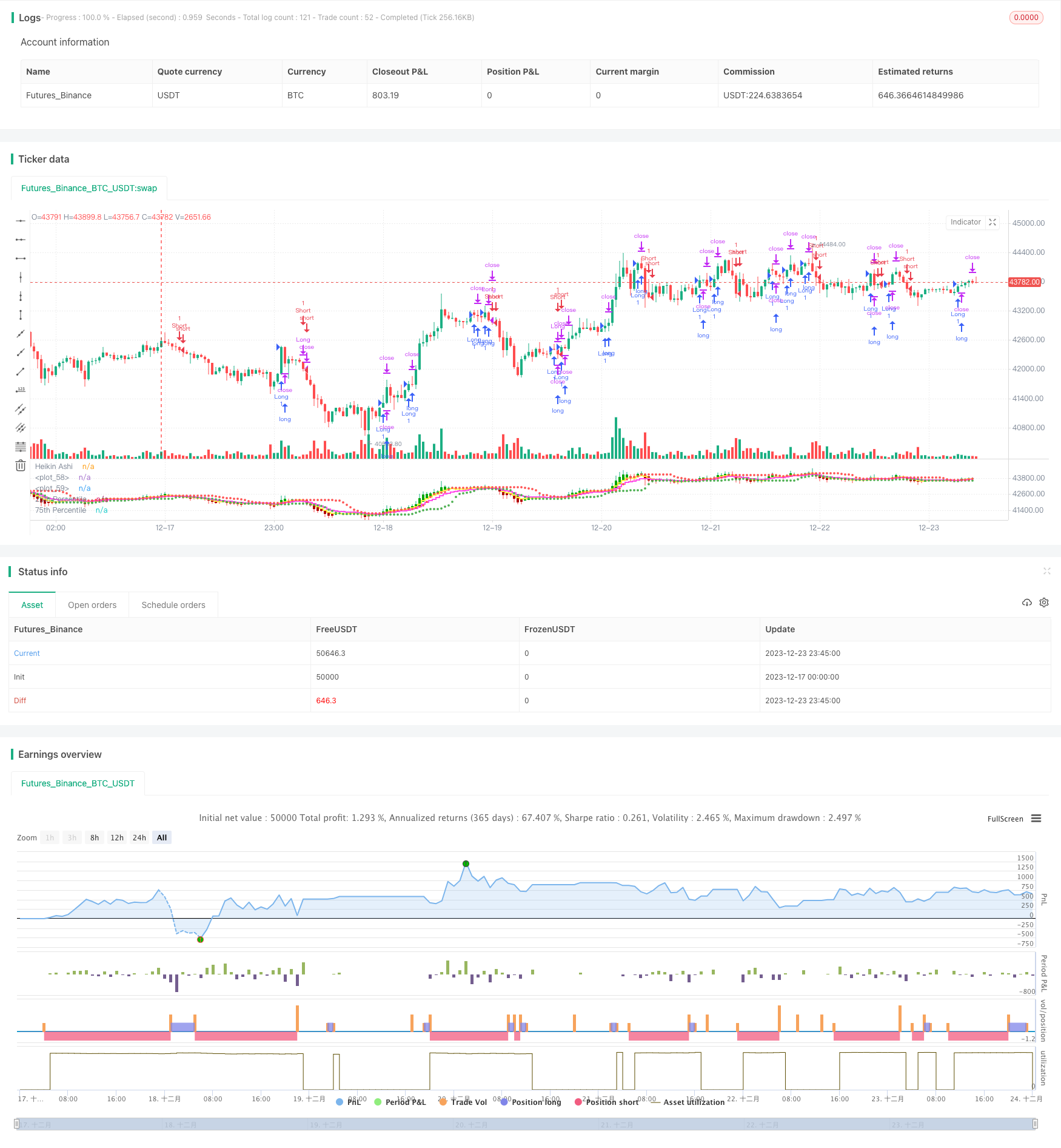
该策略基于海因阿希均线进行交易信号的生成。其中,买入和卖出信号的产生考虑到了海因阿希收盘价与75百分位价格水平的交叉以及海因阿希收盘价高于移动平均线这两个因素。
策略原理
该策略使用海因阿希均线替代普通K线进行分析,这种均线过滤掉市场噪音,更有利于发现趋势和反转信号。具体来说,该策略结合百分位数通道和移动平均线来产生交易信号:
- 当海因阿希收盘价上穿75百分位价格时产生买入信号。
- 当海因阿希收盘价下穿5日移动平均线时产生卖出信号。
此外,该策略还设定了止损距离和追踪止损来控制单边风险。
策略优势
- 使用海因阿希均线可更清晰地识别趋势,并及时发现反转信号。
- 结合百分位数通道,可确定价格是否处于“过热”或“超卖”状态,从而判断买入和卖出的时机。
- 设置止损和追踪止损有助于主动控制风险,避免超出可承受的损失。
策略风险
- 海因阿希均线本身会产生滞后,可能错过短线操作的最佳点位。
- 百分位数通道并不能完全确定价格的转折点,存在一定的假信号率。
- 止损距离设定不当可能过于宽松或过于紧绷,进而影响策略表现。
为降低上述风险,可以适当调整移动平均线周期或调整止损比例等。
策略优化
- 测试不同移动平均线组合,找到最佳参数。
- 测试不同百分位数通道参数,确保捕捉价格的“热区”。
- 结合其他指标对买卖信号进行验证,过滤假信号。
- 动态调整止损距离。
总结
本策略整合海因阿希均线、百分位数通道和移动平均线多个指标,形成交易系统。该系统能有效识别趋势方向,并设置止损来控制风险,是一个值得考量的量化交易策略。通过优化参数以及加入其他辅助指标,有望进一步提高系统的稳定性。
策略源码
/*backtest
start: 2023-12-17 00:00:00
end: 2023-12-24 00:00:00
period: 45m
basePeriod: 5m
exchanges: [{"eid":"Futures_Binance","currency":"BTC_USDT"}]
*/

//@version=5
strategy("HK Percentile Interpolation One",shorttitle = "HKPIO", overlay=false, default_qty_type = strategy.cash, default_qty_value = 5000, calc_on_order_fills = true, calc_on_every_tick = true)

// Input parameters
stopLossPercentage = input(3, title="Stop Loss (%)") // User can set Stop Loss as a percentage
trailStopPercentage = input(1.5, title="Trailing Stop (%)") // User can set Trailing Stop as a percentage
lookback = input.int(14, title="Lookback Period", minval=1) // User can set the lookback period for percentile calculation
yellowLine_length = input.int(5, "Yellow", minval=1) // User can set the length for Yellow EMA
purplLine_length = input.int(10, "Purple", minval=1) // User can set the length for Purple EMA
holdPeriod = input.int(200, title="Minimum Holding Period", minval=10) // User can set the minimum holding period
startDate = timestamp("2021 01 01")  // User can set the start date for the strategy

// Calculate Heikin Ashi values
haClose = ohlc4
var float haOpen = na
haOpen := na(haOpen[1]) ? (open + close) / 2 : (haOpen[1] + haClose[1]) / 2
haHigh = math.max(nz(haOpen, high), nz(haClose, high), high)
haLow = math.min(nz(haOpen, low), nz(haClose, low), low)

// Calculate Moving Averages
yellowLine = ta.ema(haClose, yellowLine_length)
purplLine = ta.ema(haClose, purplLine_length)

// Calculate 25th and 75th percentiles
p25 = ta.percentile_linear_interpolation(haClose, lookback, 28)
p75 = ta.percentile_linear_interpolation(haClose, lookback, 78)

// Generate buy/sell signals
longSignal = ta.crossover(haClose, p75) and haClose > yellowLine
sellSignal = ta.crossunder(haClose, yellowLine)
longSignal1 = ta.crossover(haClose, p75) and haClose > purplLine
sellSignal1 = ta.crossunder(haClose, purplLine)

// Set start time and trade conditions
if(time >= startDate)
    // When longSignal is true, enter a long trade and set stop loss and trailing stop conditions
    if (longSignal)
        strategy.entry("Long", strategy.long, 1)
        strategy.exit("Sell", "Long", stop=close*(1-stopLossPercentage/100), trail_points=close*trailStopPercentage/100, trail_offset=close*trailStopPercentage/100)
    // When sellSignal is true, close the long trade
    if (sellSignal)
        strategy.close("Long")
    // When sellSignal1 is true, enter a short trade
    if (sellSignal1)
        strategy.entry("Short", strategy.short, 1)
    // When longSignal1 is true, close the short trade
    if (longSignal1)
        strategy.close("Short")

// Plot Heikin Ashi candles
plotcandle(haOpen, haHigh, haLow, haClose, title="Heikin Ashi", color=(haClose >= haOpen ? color.rgb(1, 168, 6) : color.rgb(176, 0, 0)))

// Plot 25th and 75th percentile levels
plot(p25, title="25th Percentile", color=color.green, linewidth=1, style=plot.style_circles)
plot(p75, title="75th Percentile", color=color.red, linewidth=1, style=plot.style_circles)

// Plot Moving Averages
plot(yellowLine, color = color.rgb(254, 242, 73, 2), linewidth = 2, style = plot.style_stepline)
plot(purplLine, color = color.rgb(255, 77, 234, 2), linewidth = 2, style = plot.style_stepline)