概述
动态趋势追踪反转策略是一种基于JD Sequential指标的短期量化交易策略。该策略通过实时追踪价格的高点和低点,判断当前趋势方向和力度,实现高效捕捉市场反转点,进行进入和退出的定时。相比传统的JD Sequential策略,该策略做出了如下改进:
- 使用高点和低点判断趋势,而不是收盘价,可以更快捕捉价格变化。
- 计数器最大数为7而不是9,可以更快产生交易信号。
- 增加了支持阻力线和5计数反转作为止损的选项。
该策略适合在短线时间周期如5分钟、15分钟使用,可以有效捕捉短期价格波动和反转机会。
策略原理
动态趋势追踪反转策略的核心逻辑基于JD Sequential指标,该指标通过比较当前周期与之前两个周期的高点和低点,判断价格是否连续创出更高的高点或者更低的低点,从而给出1-7的顺序计数。当计数累计到7时产生交易信号。
具体来说,策略中定义了以下变量:
- sp_up:当高点价格超过之前第二个周期高点价格时为true
- sp_dn:当低点价格低于之前第二个周期低点价格时为true
- sp_ct: 记录当前计数,如果sp_up或sp_dn为true则+1计数,最大为7
- sp_com:计数等于7时为true
- sp_usr:计数为7且sp_up时的中价,作为上行阻力
- sp_dsr:计数为7且sp_dn时的中价,作为下行支持
交易信号的产生逻辑是:
- 长仓信号:sp_com为true且sp_dn为true,表示计数完成且处于下跌趋势
- 短仓信号:sp_com为true且sp_up为true,表示计数完成且处于上涨趋势
止损逻辑是:
- 长仓止损:计数反转为5(sp_up为true)或价格上穿sp_usr
- 短仓止损:计数反转为5(sp_dn为true)或价格下破sp_dsr
该策略通过实时比较高低点判定趋势方向和力度,计数器计时入场,可以有效捕捉短期反转机会。同时设置止损线来控制风险。
优势分析
与传统的JD Sequential策略相比,动态趋势追踪反转策略具有以下优势:
- 更快速的信号产生。使用高低点比较可以比收盘价更快捕捉趋势,7计数可以比9计数更快产生信号。
- 增加止损机制。加入5计数反转和支持阻力止损可以更好控制风险。
- 可配置灵活。可选择是否加入止损以及显示部分计数。
- 适合短线。高频率信号配合适当止损,特别适合短线时间周期。
该策略主要优势是响应迅速,可以有效捕捉短期突发事件导致的大幅波动。同时,相比完全手动交易,算法信号产生和止损可以减少交易者情绪影响,从而提高稳定性。
风险分析
动态趋势追踪反转策略也存在一定的风险:
- 高频交易增加交易成本。较高的交易频率会产生更多的手续费和滑点成本。
- 容易产生错误信号。在震荡市中,高低点的比较可能频繁触发交易信号,容易被套。
- 止损过于激进。硬止损容易被秒出,可以考虑及时移位止损。
为降低上述风险,可以从以下几个方面进行优化:
- 调整持仓规模,降低单笔交易占用资金量。
- 在震荡行情中暂停交易,避免无效交易。
- 采用移动止损或区间突破止损,减少被套盘概率。
策略优化方向
动态趋势追踪反转策略还有很大的优化空间,主要方向包括:
多时间周期组合。可以在更高时间周期确定主趋势方向,避免与主趋势对抗交易。
与其他指标组合。可以与波动率指标、成交量指标等组合,提高信号的质量。
机器学习过滤。利用机器学习算法对交易信号进行辅助判断,减少错误交易。
参数优化。可以优化计数周期数、交易时间段、持仓比例等参数,拟合不同市场条件。
增加风控机制。加入移动止损、仓位控制等更丰富的风控手段,进一步限制风险。
回测积累数据。扩大回测样本量和时间跨度,测试参数稳定性。
总结
动态趋势追踪反转策略通过实时比较高低点判断趋势方向和力度,使用JD Sequential指标的7计数规则产生交易信号,实现高频捕捉短期反转机会。相比传统JD策略,该策略做出了使用高低点判断、缩短计数周期、增加止损机制等改进,可以获得更及时的交易信号。
该策略主要优势是响应迅速,适合短线捕捉反转,同时也存在交易频繁、止损激进等风险。未来的优化方向包括参数调整、风控机制增强、多时间周期组合等。通过不断优化与迭代,该策略有望成为高效捕捉短期反转信号的有力工具。
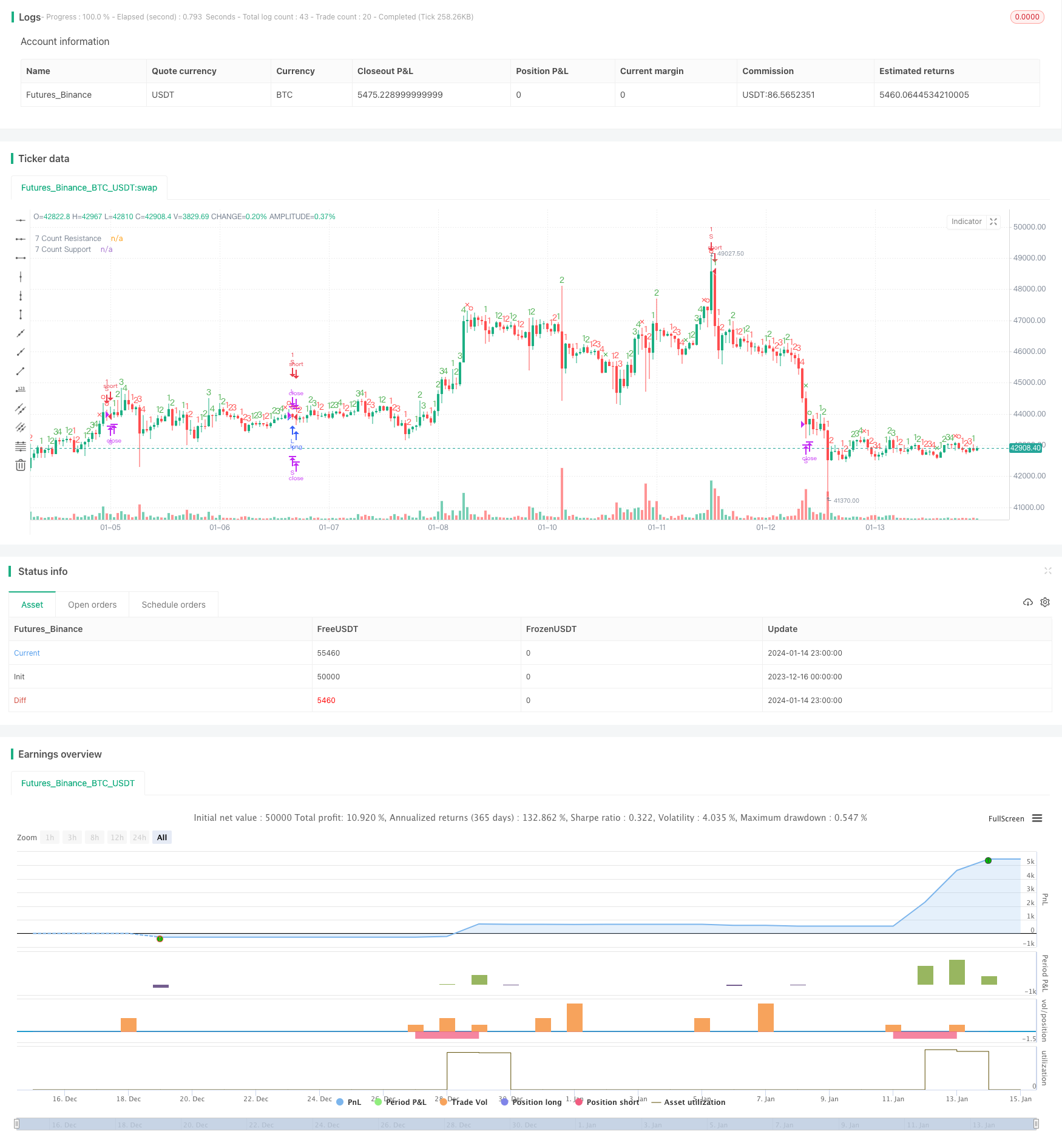
/*backtest
start: 2023-12-16 00:00:00
end: 2024-01-15 00:00:00
period: 1h
basePeriod: 15m
exchanges: [{"eid":"Futures_Binance","currency":"BTC_USDT"}]
*/

// @NeoButane 7 Dec. 2018
// JD Aggressive Sequential Setup
// Not based off official Tom DeMarke documentation. As such, I have named the indicator JD instead oF TD to reflect this, and as a joke.
//
// Difference vs. TD Sequential: faster trade exits and a unique entry. Made for low timeframes.
// - Highs or lows are compared instead of close.
// - Mirrors only the Setup aspect of TD Sequential (1-9, not to 13)
// - Count maxes out at 7 instead of 9. Also part of the joke if I'm going to be honest here

// v1 - Release - Made as a strategy, 7 count
//    . S/R on 7 count
//   .. Entry on 7 count
//  ... Exit on 5 count or S/R cross

//@version=3
title = "JD Aggressive Sequential Setup"
vers  = " 1.0 [NeoButane]"
total = title + vers
strategy(total, total, 1, 0)

xx        = input(true, "Include S/R Crosses Into Stop Loss")
show_sp   = input(true, "Show Count 1-4")
sp_ct     = 0
inc_sp(x) => nz(x) == 7 ? 1 : nz(x) + 1
sp_up     = high > high[2]
sp_dn     = low < low[2]
sp_col    = sp_up ? green : red
sp_comCol = sp_up ? red : green
sp_ct    := sp_up ? (nz(sp_up[1]) and sp_col == sp_col[1] ? inc_sp(sp_ct[1]) : 1) : sp_dn ? (nz(sp_dn[1]) and sp_col == sp_col[1] ? inc_sp(sp_ct[1]) : 1) : na
sp_com    = sp_ct == 7
sp_sr     = valuewhen(sp_ct == 5, close, 0)
sp_usr    = valuewhen(sp_ct == 7 and sp_up, sma(hlc3, 2), 0)
sp_usr   := sp_usr <= sp_usr[1] * 1.0042 and sp_usr >= sp_usr[1] * 0.9958 ? sp_usr[1] : sp_usr
sp_dsr    = valuewhen(sp_ct == 7 and sp_dn, sma(hlc3, 2), 0)
sp_dsr   := sp_dsr <= sp_dsr[1] * 1.0042 and sp_dsr >= sp_dsr[1] * 0.9958 ? sp_dsr[1] : sp_dsr
locc = location.abovebar
plotchar(show_sp and sp_ct == 1, 'Setup: 1', '1', locc, sp_col, editable=false)
plotchar(show_sp and sp_ct == 2, 'Setup: 2', '2', locc, sp_col, editable=false)
plotchar(show_sp and sp_ct == 3, 'Setup: 3', '3', locc, sp_col, editable=false)
plotchar(show_sp and sp_ct == 4, 'Setup: 4', '4', locc, sp_col, editable=false)
plotshape(sp_ct == 5, 'Setup: 5', shape.xcross, locc, sp_comCol, 0, 0, '5', sp_col)
plotshape(sp_ct == 6, 'Setup: 6', shape.circle, locc, sp_comCol, 0, 0, '6', sp_col)
plotshape(sp_ct == 7, 'Setup: 7', shape.circle, locc, sp_comCol, 0, 0, '7', sp_col)
// plot(sp_sr, "5 Count Support/Resistance", gray, 2, 6)
plot(sp_usr, "7 Count Resistance", maroon, 2, 6)
plot(sp_dsr, "7 Count Support", green, 2, 6)

long  = (sp_com and sp_dn)
short = (sp_com and sp_up)
sl_l  = xx ? crossunder(close, sp_dsr) or (sp_ct == 5 and sp_up) or short : (sp_ct == 5 and sp_up) or short
sl_s  = xx ? crossover(close, sp_usr) or (sp_ct == 5 and sp_dn) or long : (sp_ct == 5 and sp_dn) or long

strategy.entry('L', 1, when = long)
strategy.close('L', when = sl_l)
strategy.entry('S', 0, when = short)
strategy.close('S', when = sl_s)