概述
本策略的主要思想是当股票价格下跌到一定比例时,可以逐步加仓,从而达到降低平均持仓成本的目的。当价格反弹时,由于平均持仓成本更低,可以获得更高的收益。
策略原理
当股价首次上穿20日简单移动平均线时,做多开仓。如果此后股价下跌幅度达到设置的目标亏损百分比,例如10%,则加仓指定比例的头寸,例如50%的当前头寸。这样可以降低平均持仓成本。当股价达到设置的止盈点时,例如比平均持仓成本高10%,全部平仓止盈。
具体来说,strategy函数设置好参数如允许最多4次加仓,头寸计算方式为占用资金百分比,初次开仓头寸为10%。获取20日简单移动平均线,当收盘价上穿该平均线且无仓位时开多仓。然后计算持仓的浮动盈亏比例,如果达到目标亏损百分比则按目标加仓比例继续加仓,直到股票反弹止盈。
优势分析
这种策略的最大优势在于,当行情不利时,可以通过加仓降低平均持仓成本,在行情转好时获得更大收益,实现亏少赚多的效果。与简单的移动止损相比,这样的策略可以更好地把握行情,而不是在股价继续下跌后被迫止损。
同时,该策略允许多次加仓,最大程度利用行情反转的时间差,逐步调整仓位。这比一次性大量加仓的成本更低,也更符合多数投资者的资金实力。
风险分析
当然,如果行情持续走低,这样的策略也会面临重大损失的风险。特别是在熊市中,股价下跌幅度可能远超我们的想象。因此必须合理设置加仓的比例和次数,把风险控制在可承受的范围内。
同时,我们也要注意到,如果所有投资者都采用这样的策略,那么当大量投资者亏损达到目标百分比时,可能会出现集体加仓的情况。这会推高股价,形成非理性的短期反弹。如果我们不审时度势,可能会误判行情而继续加仓。结果就是izontal line当大跌再次来临时损失更重。
优化方向
这种策略可以在以下几个方面进行优化:
动态调整加仓幅度。可以根据大盘走势等情况实时调整下次加仓的比例。
结合数量指标。例如可以监测成交量明显放大来确认反转信号,避免误判。
采用跟踪止损。在加仓后采取渐进式止损,确保亏损控制在一定范围内。
总结
动态均价追踪策略通过加仓调整持仓,在保证足够资金支持的前提下,能够有效利用均价效应,在股价反转时获得超额收益。关键是要把握时点与比例,把各种风险控制在可承受的范围内。如果应用得当,这种策略可以成为量化交易中相当有效的一种方式。
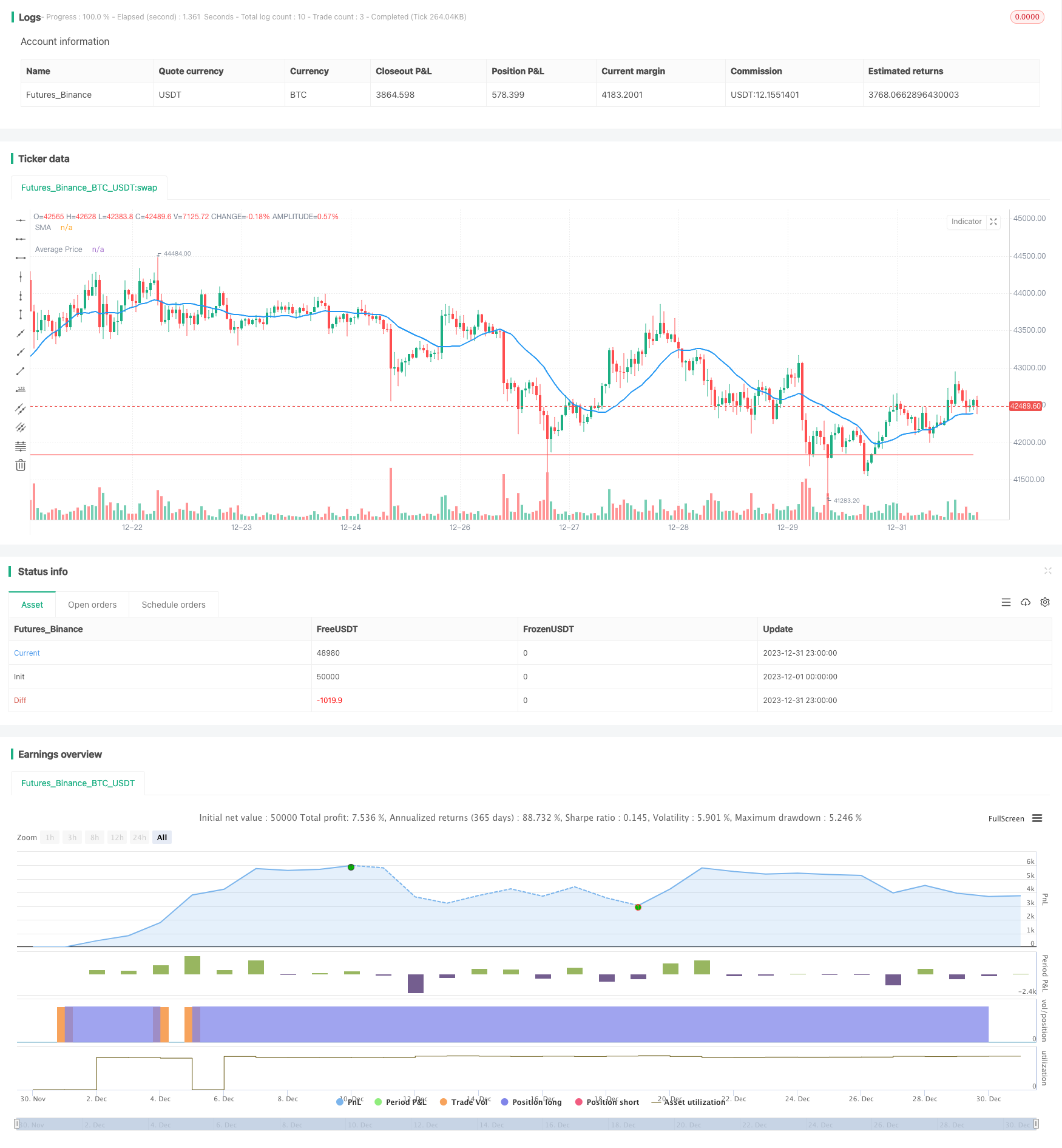
/*backtest
start: 2023-12-01 00:00:00
end: 2023-12-31 23:59:59
period: 1h
basePeriod: 15m
exchanges: [{"eid":"Futures_Binance","currency":"BTC_USDT"}]
*/

//@version=3

// ########################################################################## //
//
// This scipt is intended to demonstrate how pyramiding can be used to average
// down a position.
//
// We will buy when a stock closes above its 20 day MA and Average down if
// the trade does not go in our favor. We will hold until a profit is made.
// (which could mean we hold forever)
//
// ########################################################################## //

strategy("Average Down", overlay=true )

// Date Ranges
from_month = input(defval = 1, title = "From Month", minval = 1, maxval = 12)
from_day   = input(defval = 1, title = "From Day", minval = 1, maxval = 31)
from_year  = input(defval = 2010, title = "From Year")
to_month   = input(defval = 1, title = "To Month", minval = 1, maxval = 12)
to_day     = input(defval = 1, title = "To Day", minval = 1, maxval = 31)
to_year    = input(defval = 9999, title = "To Year")
start  = timestamp(from_year, from_month, from_day, 00, 00)  // backtest start window
finish = timestamp(to_year, to_month, to_day, 23, 59)        // backtest finish window
window = true
// Strategy Inputs
target_perc = input(-10, title='Target Loss to Average Down (%)', maxval=0)/100
take_profit = input(10, title='Target Take Profit', minval=0)/100
target_qty  = input(50, title='% Of Current Holdings to Buy', minval=0)/100
sma_period  = input(20, title='SMA Period')

// Get our SMA, this will be used for our first entry
ma = sma(close,sma_period)

// Calculate our key levels
pnl = (close - strategy.position_avg_price) / strategy.position_avg_price
take_profit_level = strategy.position_avg_price * (1 + take_profit)

// First Position
first_long = crossover(close, ma) and strategy.position_size == 0 and window
if (first_long)
    strategy.entry("Long", strategy.long)

// Average Down!
if (pnl <= target_perc)
    qty = floor(strategy.position_size * target_qty)
    strategy.entry("Long", strategy.long, qty=qty)

// Take Profit!
strategy.exit("Take Profit", "Long", limit=take_profit_level)

// Plotting
plot(ma, color=blue, linewidth=2, title='SMA')
plot(strategy.position_avg_price, style=linebr, color=red, title='Average Price')