CVD Divergence Quantitative Trading Strategy

Author: ChaoZhang, Date: 2024-03-15 16:47:47
Tags:

Strategy Overview: The CVD Divergence Quantitative Trading Strategy utilizes divergences between the CVD indicator and price to capture potential trend reversal signals. The strategy calculates the CVD indicator and compares it with price to determine if bullish or bearish divergences are formed. When a divergence signal is detected, the strategy opens a long or short position. It also uses a trailing stop loss and fixed percentage take profit to control risk and lock in profits. The strategy supports pyramiding with multiple positions.

Strategy Principles:

Calculate CVD indicator: Calculate the CVD indicator and its moving average based on bullish and bearish volume.
Identify divergences: Compare the highs and lows of the CVD indicator with the highs and lows of price to determine if divergences are formed.
- Regular bullish divergence: Price makes a lower low, but CVD forms a higher low.
- Hidden bullish divergence: Price makes a higher low, but CVD forms a lower low.
- Regular bearish divergence: Price makes a higher high, but CVD forms a lower high.
- Hidden bearish divergence: Price makes a lower high, but CVD forms a higher high.
Open positions: When a divergence signal is identified, open a long or short position based on the divergence type.
Stop loss and take profit: Use trailing stop loss and fixed percentage take profit. The stop loss price is calculated by multiplying the entry price by the stop loss percentage, and the take profit price is calculated by multiplying the entry price by the take profit percentage.
Pyramiding: The strategy allows a maximum of 3 positions for pyramiding.

Strategy Advantages:

Trend reversal signals: CVD divergence is an effective trend reversal signal that can help capture trend reversal opportunities.
Trend continuation signals: Hidden divergences can serve as trend continuation signals, helping the strategy maintain the correct direction during trends.
Risk control: By using trailing stop loss and fixed percentage take profit, risk is effectively managed.
Pyramiding: Allowing multiple positions for pyramiding enables better capitalization on trending markets.

Strategy Risks:

Signal validity: Divergence signals are not entirely reliable and false signals may occur at times.
Parameter configuration: The strategy results are sensitive to parameter settings, and different parameters may lead to different outcomes.
Stop loss slippage: In volatile markets, stop loss orders may not be filled at the predefined price, introducing additional risk.
Transaction costs: Frequent opening and closing of positions can result in high transaction costs, impacting strategy profitability.

Optimization Directions:

Dynamic parameter optimization: Employ adaptive parameters for different market conditions to improve signal validity.
Combination with other indicators: Integrate with other technical indicators such as RSI, MACD, etc., to enhance signal reliability.
Improved stop loss and take profit: Adopt more advanced stop loss and take profit strategies, such as trailing stop loss or volatility-based stop loss.
Position sizing: Dynamically adjust position sizes based on market volatility, account equity, etc.

Conclusion: The CVD Divergence Quantitative Trading Strategy aims to identify potential trend reversal opportunities by capturing divergences between the CVD indicator and price. It employs trailing stop loss and fixed percentage take profit to manage risk. The main advantages of the strategy lie in its ability to effectively capture trend reversal and continuation signals, and better capitalize on trending markets through pyramiding. However, the strategy also faces risks such as signal validity, parameter configuration, stop loss slippage, and transaction costs. Future enhancements can be made through dynamic parameter optimization, combination with other indicators, improved stop loss and take profit mechanisms, and position sizing management. Overall, the CVD Divergence Quantitative Trading Strategy is an effective and optimizable trend-following strategy suitable for quantitative traders who aim to capture trend opportunities while managing risks.

/*backtest
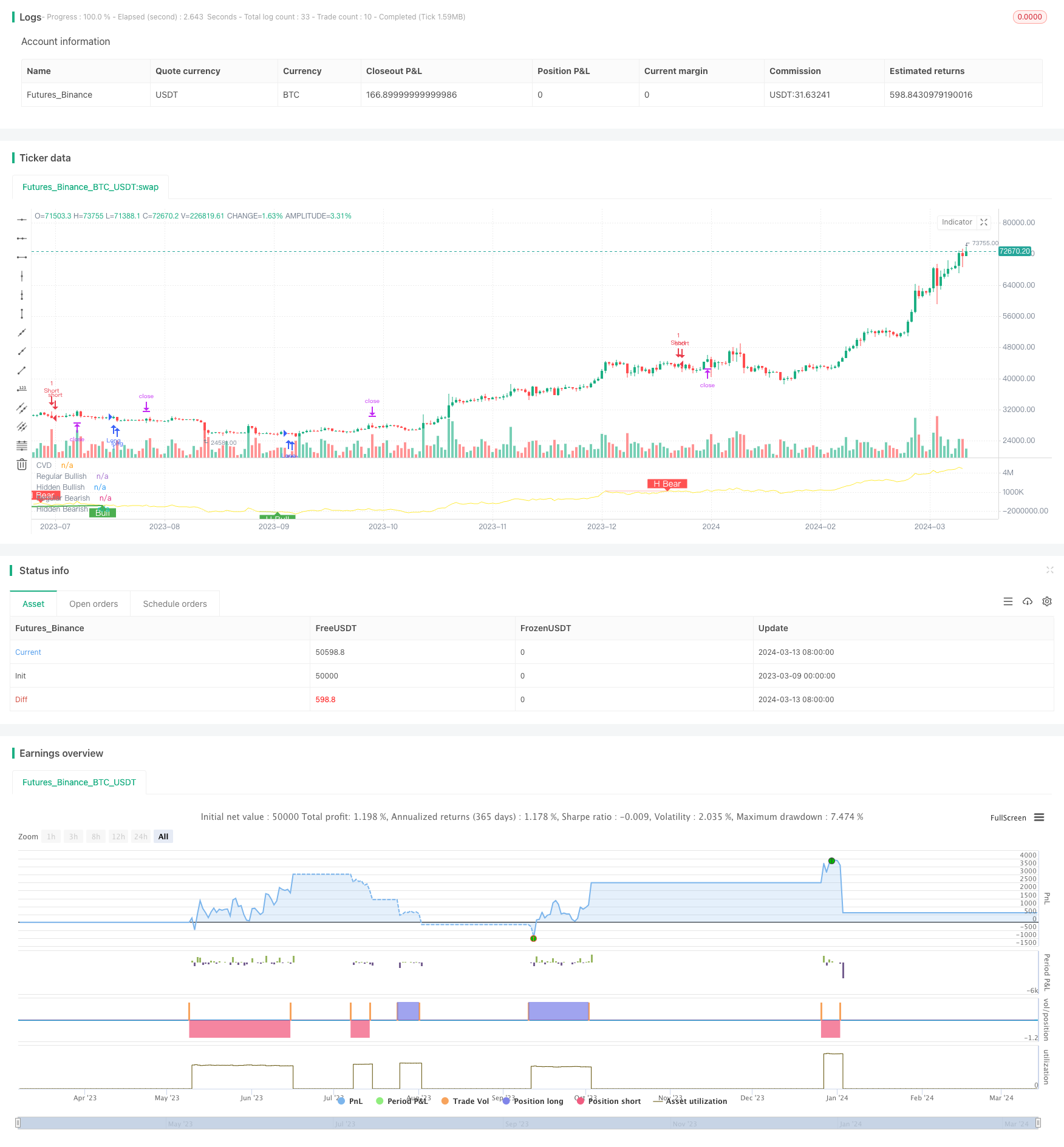
start: 2023-03-09 00:00:00
end: 2024-03-14 00:00:00
period: 1d
basePeriod: 1h
exchanges: [{"eid":"Futures_Binance","currency":"BTC_USDT"}]
*/

// This source code is subject to the terms of the Mozilla Public License 2.0 at https://mozilla.org/MPL/2.0/

//@version=5
//@ mmattman

//Thank you to @ contrerae and Tradingview each for parts of the code to make 
//this indicator and matching strategy and also theCrypster for the clean concise TP/SL code.

// indicator(title="CVD Divergence Indicator 1", shorttitle='CVD Div1', format=format.price, timeframe="", timeframe_gaps=true)

strategy("CVD Divergence Strategy.1.mm", shorttitle = 'CVD Div Str 1', overlay=false)


//..................................................................................................................
// Inputs
periodMa = input.int(title='MA Length', minval=1, defval=20)
plotMa = input(title='Plot MA?', defval=false)

// Calculations (Bull & Bear Balance Indicator by Vadim Gimelfarb)
iff_1 = close[1] < open ? math.max(high - close[1], close - low) : math.max(high - open, close - low)
iff_2 = close[1] > open ? high - low : math.max(open - close[1], high - low)
iff_3 = close[1] < open ? math.max(high - close[1], close - low) : high - open
iff_4 = close[1] > open ? high - low : math.max(open - close[1], high - low)
iff_5 = close[1] < open ? math.max(open - close[1], high - low) : high - low
iff_6 = close[1] > open ? math.max(high - open, close - low) : iff_5
iff_7 = high - close < close - low ? iff_4 : iff_6
iff_8 = high - close > close - low ? iff_3 : iff_7
iff_9 = close > open ? iff_2 : iff_8
bullPower = close < open ? iff_1 : iff_9
iff_10 = close[1] > open ? math.max(close[1] - open, high - low) : high - low
iff_11 = close[1] > open ? math.max(close[1] - low, high - close) : math.max(open - low, high - close)
iff_12 = close[1] > open ? math.max(close[1] - open, high - low) : high - low
iff_13 = close[1] > open ? math.max(close[1] - low, high - close) : open - low
iff_14 = close[1] < open ? math.max(open - low, high - close) : high - low
iff_15 = close[1] > open ? math.max(close[1] - open, high - low) : iff_14
iff_16 = high - close < close - low ? iff_13 : iff_15
iff_17 = high - close > close - low ? iff_12 : iff_16
iff_18 = close > open ? iff_11 : iff_17
bearPower = close < open ? iff_10 : iff_18

// Calculations (Bull & Bear Pressure Volume)
bullVolume = bullPower / (bullPower + bearPower) * volume
bearVolume = bearPower / (bullPower + bearPower) * volume

// Calculations Delta
delta = bullVolume - bearVolume
cvd = ta.cum(delta)
cvdMa = ta.sma(cvd, periodMa)

// Plotting
customColor = cvd > cvdMa ? color.new(color.teal, 50) : color.new(color.red, 50)
plotRef1 = plot(cvd, style=plot.style_line, linewidth=1, color=color.new(color.yellow, 0), title='CVD')
plotRef2 = plot(plotMa ? cvdMa : na, style=plot.style_line, linewidth=1, color=color.new(color.white, 0), title='CVD MA')
fill(plotRef1, plotRef2, color=customColor)
//..................................................................................................................


// len = input.int(title="RSI Period", minval=1, defval=14)
// src = input(title="RSI Source", defval=close)
lbR = input(title="Pivot Lookback Right", defval=3)
lbL = input(title="Pivot Lookback Left", defval=7)
rangeUpper = input(title="Max of Lookback Range", defval=60)
rangeLower = input(title="Min of Lookback Range", defval=5)
plotBull = input(title="Plot Bullish", defval=true)
plotHiddenBull = input(title="Plot Hidden Bullish", defval=true)
plotBear = input(title="Plot Bearish", defval=true)
plotHiddenBear = input(title="Plot Hidden Bearish", defval=true)
bearColor = color.red
bullColor = color.green
hiddenBullColor = color.new(color.green, 80)
hiddenBearColor = color.new(color.red, 80)
textColor = color.white
noneColor = color.new(color.white, 100)
osc = cvd

// plot(osc, title="CVD", linewidth=2, color=#2962FF)
// hline(50, title="Middle Line", color=#787B86, linestyle=hline.style_dotted)
// obLevel = hline(70, title="Overbought", color=#787B86, linestyle=hline.style_dotted)
// osLevel = hline(30, title="Oversold", color=#787B86, linestyle=hline.style_dotted)
// fill(obLevel, osLevel, title="Background", color=color.rgb(33, 150, 243, 90))

plFound = na(ta.pivotlow(osc, lbL, lbR)) ? false : true
phFound = na(ta.pivothigh(osc, lbL, lbR)) ? false : true
_inRange(cond) =>
	bars = ta.barssince(cond == true)
	rangeLower <= bars and bars <= rangeUpper

//------------------------------------------------------------------------------
// Regular Bullish
// Osc: Higher Low

oscHL = osc[lbR] > ta.valuewhen(plFound, osc[lbR], 1) and _inRange(plFound[1])

// Price: Lower Low

priceLL = low[lbR] < ta.valuewhen(plFound, low[lbR], 1)
bullCondAlert = priceLL and oscHL and plFound
bullCond = plotBull and bullCondAlert

plot(
     plFound ? osc[lbR] : na,
     offset=-lbR,
     title="Regular Bullish",
     linewidth=2,
     color=(bullCond ? bullColor : noneColor)
     )

plotshape(
	 bullCond ? osc[lbR] : na,
	 offset=-lbR,
	 title="Regular Bullish Label",
	 text=" Bull ",
	 style=shape.labelup,
	 location=location.absolute,
	 color=bullColor,
	 textcolor=textColor
	 )

//------------------------------------------------------------------------------
// Hidden Bullish
// Osc: Lower Low

oscLL = osc[lbR] < ta.valuewhen(plFound, osc[lbR], 1) and _inRange(plFound[1])

// Price: Higher Low

priceHL = low[lbR] > ta.valuewhen(plFound, low[lbR], 1)
hiddenBullCondAlert = priceHL and oscLL and plFound
hiddenBullCond = plotHiddenBull and hiddenBullCondAlert

plot(
	 plFound ? osc[lbR] : na,
	 offset=-lbR,
	 title="Hidden Bullish",
	 linewidth=2,
	 color=(hiddenBullCond ? hiddenBullColor : noneColor)
	 )

plotshape(
	 hiddenBullCond ? osc[lbR] : na,
	 offset=-lbR,
	 title="Hidden Bullish Label",
	 text=" H Bull ",
	 style=shape.labelup,
	 location=location.absolute,
	 color=bullColor,
	 textcolor=textColor
	 )

//------------------------------------------------------------------------------
// Regular Bearish
// Osc: Lower High

oscLH = osc[lbR] < ta.valuewhen(phFound, osc[lbR], 1) and _inRange(phFound[1])

// Price: Higher High

priceHH = high[lbR] > ta.valuewhen(phFound, high[lbR], 1)

bearCondAlert = priceHH and oscLH and phFound
bearCond = plotBear and bearCondAlert

plot(
	 phFound ? osc[lbR] : na,
	 offset=-lbR,
	 title="Regular Bearish",
	 linewidth=2,
	 color=(bearCond ? bearColor : noneColor)
	 )

plotshape(
	 bearCond ? osc[lbR] : na,
	 offset=-lbR,
	 title="Regular Bearish Label",
	 text=" Bear ",
	 style=shape.labeldown,
	 location=location.absolute,
	 color=bearColor,
	 textcolor=textColor
	 )

//------------------------------------------------------------------------------
// Hidden Bearish
// Osc: Higher High

oscHH = osc[lbR] > ta.valuewhen(phFound, osc[lbR], 1) and _inRange(phFound[1])

// Price: Lower High

priceLH = high[lbR] < ta.valuewhen(phFound, high[lbR], 1)

hiddenBearCondAlert = priceLH and oscHH and phFound
hiddenBearCond = plotHiddenBear and hiddenBearCondAlert

plot(
	 phFound ? osc[lbR] : na,
	 offset=-lbR,
	 title="Hidden Bearish",
	 linewidth=2,
	 color=(hiddenBearCond ? hiddenBearColor : noneColor)
	 )

plotshape(
	 hiddenBearCond ? osc[lbR] : na,
	 offset=-lbR,
	 title="Hidden Bearish Label",
	 text=" H Bear ",
	 style=shape.labeldown,
	 location=location.absolute,
	 color=bearColor,
	 textcolor=textColor
	 )

// alertcondition(bullCondAlert, title='Regular Bullish CVD Divergence', message="Found a new Regular Bullish Divergence, `Pivot Lookback Right` number of bars to the left of the current bar")
// alertcondition(hiddenBullCondAlert, title='Hidden Bullish CVD Divergence', message='Found a new Hidden Bullish Divergence, `Pivot Lookback Right` number of bars to the left of the current bar')
// alertcondition(bearCondAlert, title='Regular Bearish CVD Divergence', message='Found a new Regular Bearish Divergence, `Pivot Lookback Right` number of bars to the left of the current bar')
// alertcondition(hiddenBearCondAlert, title='Hidden Bearisn CVD Divergence', message='Found a new Hidden Bearisn Divergence, `Pivot Lookback Right` number of bars to the left of the current bar')

le = bullCondAlert or hiddenBullCondAlert

se = bearCondAlert or hiddenBearCondAlert

ltp = se

stp = le

// Check if the entry conditions for a long position are met
if (le) //and (close > ema200)
    strategy.entry("Long", strategy.long, comment="EL")

 // Check if the entry conditions for a short position are met
if (se) //and (close < ema200)
    strategy.entry("Short", strategy.short, comment="ES")

// Close long position if exit condition is met
if (ltp) // or (close < ema200)
    strategy.close("Long", comment="XL")

    // Close short position if exit condition is met
if (stp) //or (close > ema200)
    strategy.close("Short", comment="XS")


// The Fixed Percent Stop Loss Code
// User Options to Change Inputs (%)
stopPer = input.float(5.0, title='Stop Loss %') / 100
takePer = input.float(10.0, title='Take Profit %') / 100

// Determine where you've entered and in what direction
longStop = strategy.position_avg_price * (1 - stopPer)
shortStop = strategy.position_avg_price * (1 + stopPer)
shortTake = strategy.position_avg_price * (1 - takePer)
longTake = strategy.position_avg_price * (1 + takePer)

if strategy.position_size > 0 
    strategy.exit("Close Long", "Long", stop=longStop, limit=longTake)
if strategy.position_size < 0 
    strategy.exit("Close Short", "Short", stop=shortStop, limit=shortTake)

More

Forums
|
API
|
Github
|
About
|
SiteMap