策略概述
Kuberan策略是由Kathir编写的一款强大的交易策略。它融合了多种分析技术,形成了一个独特而强大的交易方法。该策略以财富之神Kuberan命名,象征着其丰富交易者投资组合的目标。
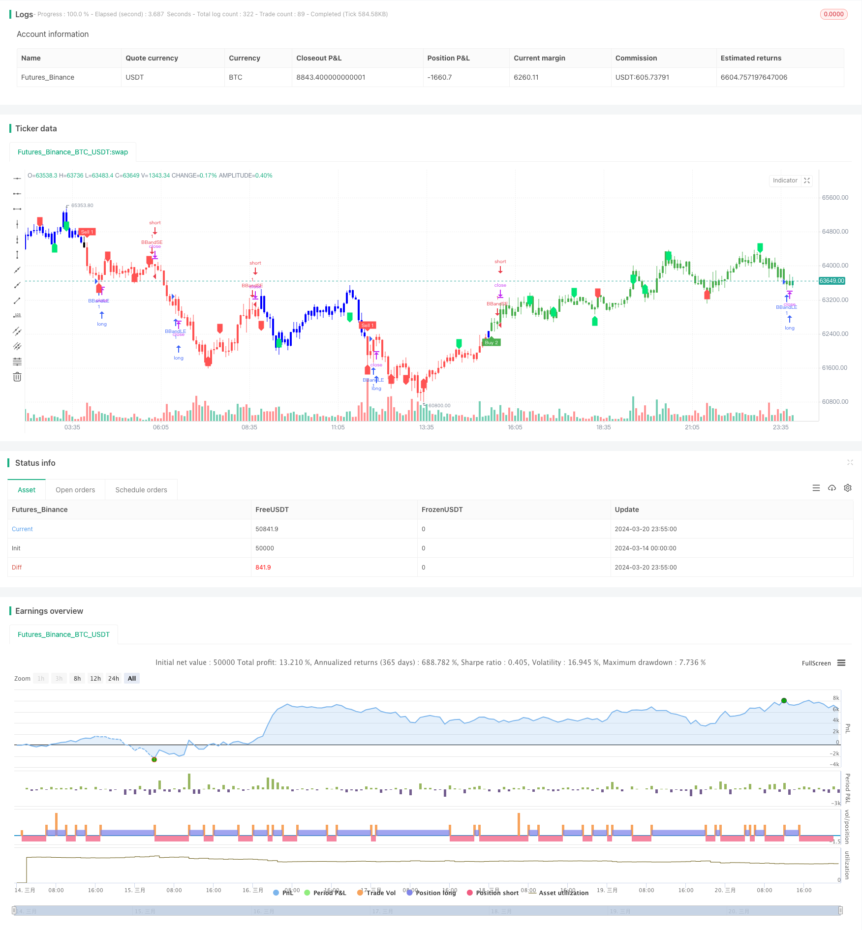
Kuberan不仅仅是一个策略,更是一个全面的交易系统。它结合了趋势分析、动量指标和成交量指标,以识别高概率的交易机会。通过利用这些要素的协同作用,Kuberan提供了明确的进场和出场信号,适用于各种水平的交易者。
策略原理
Kuberan策略的核心是多指标交汇原理。它利用了一种独特的指标组合,这些指标相互配合,以减少噪音和错误信号。具体来说,该策略使用了以下几个关键组件:
- 趋势方向判断:通过比较当前价格与支撑位和阻力位,判断当前趋势方向。
- 支撑阻力位:通过zigzag指标和枢轴点来识别关键的支撑位和阻力位。
- 背离判断:通过比较价格走势与动量指标,判断是否出现背离,提示潜在的趋势反转。
- 波动率自适应:通过ATR指标动态调整止损位,以适应不同的市场波动率。
- K线型态判断:通过特定的K线组合来确认趋势和反转信号。
通过综合考虑以上因素,Kuberan策略能够在各种市场环境下自适应调整,捕捉高概率的交易机会。
策略优势
- 多指标交汇:Kuberan策略利用了多个指标的协同作用,大大提高了信号的可靠性,降低了噪音干扰。
- 自适应性强:通过动态调整参数,该策略能够适应多变的市场环境,不易失效。
- 明确信号:Kuberan提供清晰的进场和出场信号,简化了交易决策过程。
- 回测稳健:该策略经过了严格的历史回测,在各种市场行情下都表现稳健。
- 适用性广:Kuberan适用于多种市场和品种,不限于特定交易标的。
策略风险
- 参数敏感:Kuberan策略的表现对参数选择较为敏感,不当的参数可能导致表现下降。
- 突发事件:该策略主要基于技术面信号,对基本面突发事件的应对能力有限。
- 过拟合风险:如果在参数优化时考虑过多的历史数据,可能导致策略过于迎合过去,而对未来行情适应性下降。
- 杠杆风险:如果使用过高杠杆,遭遇较大回撤时有爆仓风险。
针对以上风险,可以采取适当的控制措施,如定期调整参数、设置合理止损、适度控制杠杆、关注基本面变化等。
优化方向
- 机器学习优化:可以引入机器学习算法来动态优化策略参数,提高适应性。
- 加入基本面因素:考虑将基本面分析纳入交易决策,以应对技术面信号失效的情况。
- 投资组合管理:在资金管理层面,可以将Kuberan策略纳入投资组合,与其他策略形成有效对冲。
- 细分市场优化:针对不同市场品种的特点,定制优化策略参数。
- 高频化改造:将策略改造为高频交易版本,捕捉更多短线交易机会。
总结
Kuberan是一款功能强大,安全可靠的交易策略。它巧妙地融合了多种技术分析方法,通过指标交汇原理,在捕捉趋势和把握转折点方面表现出色。尽管任何策略都难免面临风险,但Kuberan已经在回测中证明了其稳健性,通过适当的风险控制和优化措施,相信该策略能够帮助交易者在市场博弈中掌控先机,驱动投资组合的长期稳健增长。
策略源码
/*backtest
start: 2024-03-14 00:00:00
end: 2024-03-21 00:00:00
period: 5m
basePeriod: 1m
exchanges: [{"eid":"Futures_Binance","currency":"BTC_USDT"}]
*/

// This source code is subject to the terms of the Mozilla Public License 2.0 at https://mozilla.org/MPL/2.0/
// © LonesomeThecolor.blue
// This source code is subject to the terms of the Mozilla Public License 2.0 at https://mozilla.org/MPL/2.0/
// © LonesomeThecolor.blue

//@version=5
strategy('Kuberan*', overlay=true, max_lines_count=500)
lb = input.int(5, title='Left Bars', minval=1)
rb = input.int(5, title='Right Bars', minval=1)
showsupres = input.bool(false, title='Support/Resistance', inline='srcol')
supcol = input.color(color.lime, title='', inline='srcol')
rescol = input.color(color.red, title='', inline='srcol')
// srlinestyle = input(line.style_dotted, title='Line Style/Width', inline='style')
srlinewidth = input.int(3, title='', minval=1, maxval=5, inline='style')
changebarcol = input.bool(true, title='Change Bar Color', inline='bcol')
bcolup = input.color(color.blue, title='', inline='bcol')
bcoldn = input.color(color.black, title='', inline='bcol')

ph = ta.pivothigh(lb, rb)
pl = ta.pivotlow(lb, rb)

iff_1 = pl ? -1 : na  // Trend direction
hl = ph ? 1 : iff_1
iff_2 = pl ? pl : na  // similar to zigzag but may have multTLiple highs/lows
zz = ph ? ph : iff_2
valuewhen_1 = ta.valuewhen(hl, hl, 1)
valuewhen_2 = ta.valuewhen(zz, zz, 1)
zz := pl and hl == -1 and valuewhen_1 == -1 and pl > valuewhen_2 ? na : zz
valuewhen_3 = ta.valuewhen(hl, hl, 1)
valuewhen_4 = ta.valuewhen(zz, zz, 1)
zz := ph and hl == 1 and valuewhen_3 == 1 and ph < valuewhen_4 ? na : zz

valuewhen_5 = ta.valuewhen(hl, hl, 1)
valuewhen_6 = ta.valuewhen(zz, zz, 1)
hl := hl == -1 and valuewhen_5 == 1 and zz > valuewhen_6 ? na : hl
valuewhen_7 = ta.valuewhen(hl, hl, 1)
valuewhen_8 = ta.valuewhen(zz, zz, 1)
hl := hl == 1 and valuewhen_7 == -1 and zz < valuewhen_8 ? na : hl
zz := na(hl) ? na : zz

findprevious() =>  // finds previous three points (b, c, d, e)
    ehl = hl == 1 ? -1 : 1
    loc1 = 0.0
    loc2 = 0.0
    loc3 = 0.0
    loc4 = 0.0
    xx = 0
    for x = 1 to 1000 by 1
        if hl[x] == ehl and not na(zz[x])
            loc1 := zz[x]
            xx := x + 1
            break
    ehl := hl
    for x = xx to 1000 by 1
        if hl[x] == ehl and not na(zz[x])
            loc2 := zz[x]
            xx := x + 1
            break
    ehl := hl == 1 ? -1 : 1
    for x = xx to 1000 by 1
        if hl[x] == ehl and not na(zz[x])
            loc3 := zz[x]
            xx := x + 1
            break
    ehl := hl
    for x = xx to 1000 by 1
        if hl[x] == ehl and not na(zz[x])
            loc4 := zz[x]
            break
    [loc1, loc2, loc3, loc4]

float a = na
float b = na
float c = na
float d = na
float e = na
if not na(hl)
    [loc1, loc2, loc3, loc4] = findprevious()
    a := zz
    b := loc1
    c := loc2
    d := loc3
    e := loc4
    e

_hh = zz and a > b and a > c and c > b and c > d
_ll = zz and a < b and a < c and c < b and c < d
_hl = zz and (a >= c and b > c and b > d and d > c and d > e or a < b and a > c and b < d)
_lh = zz and (a <= c and b < c and b < d and d < c and d < e or a > b and a < c and b > d)

plotshape(_hl, title='Higher Low', style=shape.labelup, color=color.new(color.lime, 0), textcolor=color.new(color.black, 0), location=location.belowbar, offset=-rb)
plotshape(_hh, title='Higher High', style=shape.labeldown, color=color.new(color.lime, 0), textcolor=color.new(color.black, 0), location=location.abovebar, offset=-rb)
plotshape(_ll, title='Lower Low', style=shape.labelup, color=color.new(color.red, 0), textcolor=color.new(color.white, 0), location=location.belowbar, offset=-rb)
plotshape(_lh, title='Lower High', style=shape.labeldown, color=color.new(color.red, 0), textcolor=color.new(color.white, 0), location=location.abovebar, offset=-rb)

float res = na
float sup = na
res := _lh ? zz : res[1]
sup := _hl ? zz : sup[1]

int trend = na
iff_3 = close < sup ? -1 : nz(trend[1])
trend := close > res ? 1 : iff_3

res := trend == 1 and _hh or trend == -1 and _lh ? zz : res
sup := trend == 1 and _hl or trend == -1 and _ll ? zz : sup
rechange = res != res[1]
suchange = sup != sup[1]

var line resline = na
var line supline = na
if showsupres
    if rechange
        line.set_x2(resline, bar_index)
        line.set_extend(resline, extend=extend.none)
        resline := line.new(x1=bar_index - rb, y1=res, x2=bar_index, y2=res, color=rescol, extend=extend.right, style=line.style_dotted, width=srlinewidth)
        resline

    if suchange
        line.set_x2(supline, bar_index)
        line.set_extend(supline, extend=extend.none)
        supline := line.new(x1=bar_index - rb, y1=sup, x2=bar_index, y2=sup, color=supcol, extend=extend.right, style=line.style_dotted, width=srlinewidth)
        supline

iff_4 = trend == 1 ? bcolup : bcoldn
barcolor(color=changebarcol ? iff_4 : na)


// Inputs
A1 = input(5, title='Key Value. \'This changes the sensitivity\' for sell1')
C1 = input(400, title='ATR Period for sell1')
A2 = input(6, title='Key Value. \'This changes the sensitivity\' for buy2')
C2 = input(1, title='ATR Period for buy2')
h = input(false, title='Signals from Heikin Ashi Candles')

xATR1 = ta.atr(C1)
xATR2 = ta.atr(C2)
nLoss1 = A1 * xATR1
nLoss2 = A2 * xATR2

src = h ? request.security(ticker.heikinashi(syminfo.tickerid), timeframe.period, close, lookahead=barmerge.lookahead_off) : close

xATRTrailingStop1 = 0.0
iff_5 = src > nz(xATRTrailingStop1[1], 0) ? src - nLoss1 : src + nLoss1
iff_6 = src < nz(xATRTrailingStop1[1], 0) and src[1] < nz(xATRTrailingStop1[1], 0) ? math.min(nz(xATRTrailingStop1[1]), src + nLoss1) : iff_5
xATRTrailingStop1 := src > nz(xATRTrailingStop1[1], 0) and src[1] > nz(xATRTrailingStop1[1], 0) ? math.max(nz(xATRTrailingStop1[1]), src - nLoss1) : iff_6

xATRTrailingStop2 = 0.0
iff_7 = src > nz(xATRTrailingStop2[1], 0) ? src - nLoss2 : src + nLoss2
iff_8 = src < nz(xATRTrailingStop2[1], 0) and src[1] < nz(xATRTrailingStop2[1], 0) ? math.min(nz(xATRTrailingStop2[1]), src + nLoss2) : iff_7
xATRTrailingStop2 := src > nz(xATRTrailingStop2[1], 0) and src[1] > nz(xATRTrailingStop2[1], 0) ? math.max(nz(xATRTrailingStop2[1]), src - nLoss2) : iff_8

pos1 = 0
iff_9 = src[1] > nz(xATRTrailingStop1[1], 0) and src < nz(xATRTrailingStop1[1], 0) ? -1 : nz(pos1[1], 0)
pos1 := src[1] < nz(xATRTrailingStop1[1], 0) and src > nz(xATRTrailingStop1[1], 0) ? 1 : iff_9

pos2 = 0
iff_10 = src[1] > nz(xATRTrailingStop2[1], 0) and src < nz(xATRTrailingStop2[1], 0) ? -1 : nz(pos2[1], 0)
pos2 := src[1] < nz(xATRTrailingStop2[1], 0) and src > nz(xATRTrailingStop2[1], 0) ? 1 : iff_10

xcolor1 = pos1 == -1 ? color.red : pos1 == 1 ? color.green : color.blue
xcolor2 = pos2 == -1 ? color.red : pos2 == 1 ? color.green : color.blue

ema1 = ta.ema(src, 1)
ema2 = ta.ema(src, 1)
above1 = ta.crossover(ema1, xATRTrailingStop1)
below1 = ta.crossover(xATRTrailingStop1, ema1)
above2 = ta.crossover(ema2, xATRTrailingStop2)
below2 = ta.crossover(xATRTrailingStop2, ema2)

buy1 = src > xATRTrailingStop1 and above1
sell1 = src < xATRTrailingStop1 and below1
buy2 = src > xATRTrailingStop2 and above2
sell2 = src < xATRTrailingStop2 and below2

barbuy1 = src > xATRTrailingStop1
barsell1 = src < xATRTrailingStop1
barbuy2 = src > xATRTrailingStop2
barsell2 = src < xATRTrailingStop2

// plotshape(buy1, title="Buy 1", text='Buy 1', style=shape.labelup, location=location.belowbar, color=color.green, textcolor=color.white, transp=0, size=size.tiny)
plotshape(sell1, title='Sell 1', text='Sell 1', style=shape.labeldown, location=location.abovebar, color=color.new(color.red, 0), textcolor=color.new(color.white, 0), size=size.tiny)
plotshape(buy2, title='Buy 2', text='Buy 2', style=shape.labelup, location=location.belowbar, color=color.new(color.green, 0), textcolor=color.new(color.white, 0), size=size.tiny)
// plotshape(sell2, title="Sell 2", text='Sell 2', style=shape.labeldown, location=location.abovebar, color=color.red, textcolor=color.white, transp=0, size=size.tiny)

// barcolor(barbuy1 ? color.green : na)
barcolor(barsell1 ? color.red : na)
barcolor(barbuy2 ? color.green : na)
// barcolor(barsell2 ? color.red : na)

// alertcondition(buy1, "UT Long 1", "UT Long 1")
alertcondition(sell1, 'UT Short 1', 'UT Short 1')
alertcondition(buy2, 'UT Long 2', 'UT Long 2')

// strategy.entry('long', strategy.long, when=buy2)
source = close
length = input.int(20, minval=1)
mult = input.float(2.0, minval=0.001, maxval=50)
basis = ta.sma(source, length)
dev = mult * ta.stdev(source, length)
upper = basis + dev
lower = basis - dev
buyEntry = ta.crossover(source, lower)
sellEntry = ta.crossunder(source, upper)
if (ta.crossover(source, lower) )
	strategy.entry("BBandLE", strategy.long, stop=lower, oca_name="BollingerBands",  comment="BBandLE")
else
	strategy.cancel(id="BBandLE")
if (ta.crossunder(source, upper))
	strategy.entry("BBandSE", strategy.short, stop=upper, oca_name="BollingerBands",comment="BBandSE")
else
	strategy.cancel(id="BBandSE")
//plot(strategy.equity, title="equity", color=color.red, linewidth=2, style=plot.style_areabr)

lengthTL = input.int(14, 'Swing Detection Lookback')
multTL = input.float(1., 'Slope', minval = 0, step = .1)
calcMethod = input.string('Atr', 'Slope Calculation Method', options = ['Atr','Stdev','Linreg'])
backpaint = input(true, tooltip = 'Backpainting offset displayed elements in the past. Disable backpainting to see real time information returned by the indicator.')

//Style
upCss = input.color(color.teal, 'Up Trendline Color', group = 'Style')
dnCss = input.color(color.red, 'Down Trendline Color', group = 'Style')
showExt = input(true, 'Show Extended Lines')

//-----------------------------------------------------------------------------}
//Calculations
//-----------------------------------------------------------------------------{
var upperTL = 0.
var lowerTL = 0.
var slope_phTL = 0.
var slope_plTL = 0.

var offset = backpaint ? lengthTL : 0

n = bar_index
srcTL = close

phTL = ta.pivothigh(lengthTL, lengthTL)
plTL = ta.pivotlow(lengthTL, lengthTL)

//Slope Calculation Method
slope = switch calcMethod
    'Atr'    => ta.atr(lengthTL) / lengthTL * multTL
    'Stdev'  => ta.stdev(srcTL,lengthTL) / lengthTL * multTL
    'Linreg' => math.abs(ta.sma(srcTL * n, lengthTL) - ta.sma(srcTL, lengthTL) * ta.sma(n, lengthTL)) / ta.variance(n, lengthTL) / 2 * multTL

//Get slopes and calculate trendlines
slope_phTL := phTL ? slope : slope_phTL
slope_plTL := plTL ? slope : slope_plTL

upperTL := phTL ? phTL : upperTL - slope_phTL
lowerTL := pl ? pl : lowerTL + slope_plTL

var upos = 0
var dnos = 0
upos := phTL ? 0 : close > upperTL - slope_phTL * lengthTL ? 1 : upos
dnos := pl ? 0 : close < lowerTL + slope_plTL * lengthTL ? 1 : dnos