
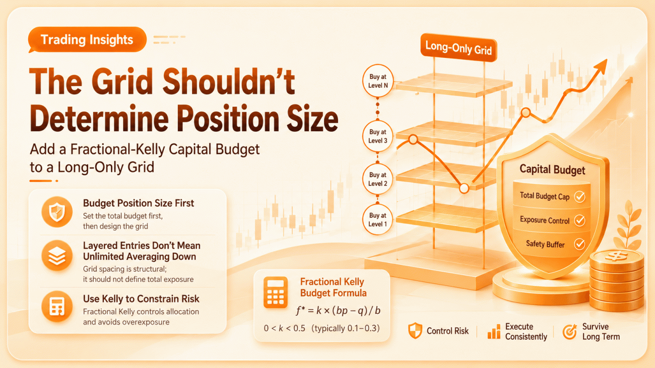
A grid answers the question, “At what price should the strategy take an action?” Kelly answers a different question: “How much capital may the entire strategy use at most?” Only by separating these two responsibilities can a grid evolve from a set of averaging-down rules into a system that can be backtested, reconciled, and knows when it should stop taking additional risk.
This article discusses a long-only dynamic grid prototype for linear perpetual contracts supported by FMZ. It can be used with traditional crypto assets, and it can also be used to study TradFi-mapped perpetual products such as NVDA, without relying on any exchange-specific private interface.
First, a boundary condition: this article presents the strategy architecture and an FMZ engineering implementation. It makes no promise of profitability, nor does it use an attractive in-sample equity curve as a substitute for out-of-sample validation. A grid strategy accumulates inventory during prolonged declines, while Kelly estimates are themselves affected by sampling error. Combining the two does not automatically produce a low-risk strategy.
The strategy is only an implementation of the ideas discussed in this article and should be treated as a research prototype. It may require further upgrades and revisions. It is intended solely for learning and discussion.
Strategy source code: https://www.fmz.com/strategy/547981
1. What I Really Want to Solve Is Not “How Wide Should the Grid Be?”
When people build grid strategies, it is easy to focus almost entirely on grid spacing: 0.5% or 1%, five levels or ten, equal spacing or exponential spacing.
But what determines whether the strategy can survive is often not one of those parameters. It is a more fundamental question:
If price keeps falling, how much capital is this entire grid allowed to consume at most?
Traditional grids often tie “how much to buy at each level” directly to “how far price has fallen.” One contract on the first level, two on the second, four on the third. On the surface, this seems to optimize the average entry price. In practice, it automatically expands the risk budget as price moves against the strategy.
This prototype deliberately separates these responsibilities:
- The grid layer decides when to buy and when to exit.
- The Kelly layer decides the total fraction of capital that the entire grid is currently allowed to use.
- The execution layer converts a quote-currency budget into contract quantity and handles partial fills and order reconciliation.
- The risk-control layer has the authority to stop adding new risk and, when necessary, exit positions batch by batch.
The grid is not allowed to increase the total budget on its own. Even if price crosses five grid levels in succession, the combined capital allocated to those five levels may not exceed the ceiling provided by the Kelly layer.
2. Why the Strategy Is Long-Only
This is not based on the assumption that “long-only always makes money.” The purpose of the strategy is to study a specific structure: on assets for which there is a hypothesis of long-term positive drift, use a pullback grid to improve entries and exits instead of maintaining two opposing inventories at the same time.
For stock-mapped perpetuals such as NVDA, that hypothesis may come from the possibility of long-term growth in the underlying company’s value. For major crypto assets, it comes from a different and less stable assumption about long-term adoption. In either case, positive drift is a hypothesis to be tested, not a law of nature.
Long-only also does not mean “always keep buying.” The prototype requires:
text
FastEMA >= SlowEMA
and Close >= SlowEMA
Only when this bullish regime is satisfied may the strategy add new grid positions. When price crosses downward through a grid level, the strategy buys. If price later rebounds by one entry-time grid spacing, the corresponding batch is closed.
Each batch has its own actual average fill price and exit target:
            text

            TargetPrice = ActualEntryPrice × (1 + EntrySpacing)
There is an easily overlooked detail here: once a batch has been filled, its target is no longer modified by ATR.
ATR may change grid levels that have not yet been filled, but it must not retroactively alter the plan of a trade that is already carrying risk. Otherwise, when volatility expands, the take-profit line keeps moving farther away, and a dynamic parameter becomes an excuse to postpone exits.
The anchor is also allowed to move upward only when the strategy is flat, has no active order, and the trend is healthy. While holding positions, the anchor does not chase price downward. This prevents the grid from moving its “reference starting point” lower and lower during a decline until even the hard-stop benchmark loses its meaning.
3. Grid Spacing Should Cover Costs Before It Tries to Model Volatility
If the grid is too narrow, the trade count may look impressive, but gross profit can be completely consumed by fees and slippage. If the grid is too wide, the strategy may remain inactive for a long time.
The prototype defines grid spacing as the maximum of three constraints:
            text

            Spacing = clamp(
    max(
        MinGridPct,
        ATR / Price × AtrMultiplier,
        2 × (FeePerSide + SlippagePerSide) × CostFloorMultiple
    ),
    MinGridPct,
    MaxGridPct
)
The three components answer three different questions:
- What is the minimum operational grid spacing the strategy is willing to use?
- What is the current scale of market volatility?
- Given the estimated cost of one entry plus one exit, how much safety margin should be left?
Suppose one-way fees and slippage are both estimated at 0.05%, and the safety multiple is 2. Then the cost floor is:
            text

            2 × (0.05% + 0.05%) × 2 = 0.4%
Even if ATR becomes temporarily very low, the grid will not shrink below 0.4%.
This does not guarantee that every completed trade will be profitable. It simply avoids designing a grid whose expected gross spread is already smaller than its assumed transaction costs.
4. Do Not Use the “Win Rate of Completed Grid Trades” to Calculate Kelly
This is the most important part of the entire design.
A grid trade that has completed is usually a small winner. The inventory with the largest losses is often precisely the inventory that has not yet completed.
If we count only batches that have already exited, we can easily obtain data like this:
            text

            Completed grid trades: 93
Winning trades:        90
Losing trades:          3
Win rate:             96.8%
If that win rate is then plugged into the classic binary Kelly formula, the result may recommend an extremely aggressive position size.
The problem is that the unrealized losses still sitting in the account are excluded from the sample.
The strategy is hiding unrealized losses outside the statistical sample and then using a selectively inflated win rate to guide position sizing. That is a textbook form of self-deception.
For this reason, the prototype does not treat “one completed grid cycle” as a Kelly event. Instead, it periodically samples mark-to-market equity, including unrealized PnL:
            text

            EquityReturn = Equity_t / Equity_(t-1) - 1

AverageExposure =
    (ExposureFraction_t + ExposureFraction_(t-1)) / 2

UnitRiskReturn = EquityReturn / AverageExposure
ExposureFraction is the current notional exposure divided by a fixed reference equity.
The purpose is to normalize equity changes observed under different position sizes into something closer to the empirical return distribution generated by one unit of risk exposure.
Instead of using the simplified Kelly formula designed for a binary gamble, the prototype searches directly over historical empirical samples:
            text

            f_raw = argmax mean(log(1 + f × UnitRiskReturn))
        f ∈ [0, 1]
If a candidate f would make 1 + f × r <= 0 for any observation, that candidate is invalid.
If the average log growth of every positive-position candidate is no better than staying flat, the optimum becomes:
            text

            f_raw = 0
That still does not mean the estimate is reliable enough to use directly. The actual allocation is discounted further:
            text

            Confidence = min(1, SampleCount / (2 × MinSamples))

f_used = min(
    MaxStrategyEquityPct,
    f_raw × KellyFraction × Confidence
)
By default, the prototype uses one-quarter Kelly:
            text

            KellyFraction = 0.25
When the sample count has only just reached the minimum requirement, the confidence multiplier is still only 0.5. The discount is gradually relaxed only as more valid samples accumulate.
Before there are enough Kelly samples, the strategy uses a small warm-up allocation.
Without that step, the strategy would fall into a paradox: without exposure there are no strategy-return samples, and without samples the strategy would never be allowed to create exposure.
5. Kelly Controls the Total Budget, Not Each Individual Grid Level
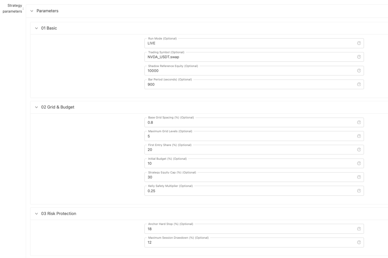
Assume the fixed reference equity is 100,000 USDT and the warm-up allocation is 10%. The entire grid is therefore allowed a maximum notional budget of 10,000 USDT during the warm-up phase.
The five grid levels do not increase in size as price falls. Instead, their weights decrease by a factor of 0.85:
            text

            1.0000, 0.8500, 0.7225, 0.6141, 0.5220
After normalization, the allocation looks approximately like this:
| Level | Budget Weight | Approx. Share of Total Budget | Example Warm-Up Budget |
|---|---|---|---|
| 1 | 1.0000 | 26.96% | 2696 USDT |
| 2 | 0.8500 | 22.92% | 2292 USDT |
| 3 | 0.7225 | 19.49% | 1949 USDT |
| 4 | 0.6141 | 16.56% | 1656 USDT |
| 5 | 0.5220 | 14.08% | 1408 USDT |
This design is not claiming that deeper grid levels are inherently “safer.” It is explicitly rejecting the traditional Martingale structure: the more adverse the price movement becomes, the smaller the incremental risk added by each new level.
Suppose the later empirical return distribution produces:
            text

            f_raw = 40%
and the one-quarter Kelly multiplier is 0.25, while the current confidence discount is 0.75:
            text

            f_used = 40% × 0.25 × 0.75 = 7.5%
The total grid budget is now reduced to 7,500 USDT.
If existing notional exposure is clearly above the new budget plus a rebalancing buffer, the strategy reduces positions batch by batch, starting with deeper lots, rather than continuing to wait for every batch to reach its original take-profit target.
One point deserves emphasis: reducing exposure when the Kelly estimate falls also creates turnover and slippage. A buffer is therefore important. A noisy estimator should not trigger a trade every time it changes slightly.
6. Converting a Quote-Currency Budget into FMZ Contract Quantity
The strategy interface takes a capital budget as input, while the amount passed to an FMZ contract order is usually the number of contracts.
You cannot simply pass 1,000 USDT as the amount argument of an order function.
The prototype uses exchange.GetMarkets() to inspect market metadata, focusing on:
CtVal: how much base asset each contract represents;CtValCcy: the currency in which the contract value is expressed;AmountSize: quantity precision or step size;MinQty: minimum order quantity;MinNotional: minimum notional value.
Version v0.1.0 accepts only linear contracts for which CtValCcy is the base asset.
In that case, the quantity can be estimated as:
            text

            RawAmount = QuoteBudget / (Price × CtVal)
Amount = floor_to_step(RawAmount, AmountStep)
After rounding the quantity downward to the valid step size, the strategy checks the minimum quantity and minimum notional requirements.
If the contract-value unit cannot be confirmed, the strategy refuses to start instead of guessing how the conversion should work.
The symbol also uses the full FMZ format, for example:
            text

            BTC_USDT.swap
When researching stock-mapped perpetuals, this only needs to be replaced with the actual full symbol provided by the target FMZ exchange.
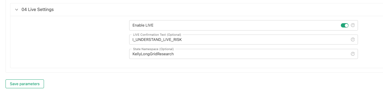
The strategy itself does not switch exchanges, modify leverage, change isolated/cross-margin settings, alter one-way/hedge position modes, or pass exchange-specific order parameters inside the code.
7. The Hard Part Is Not the Formula — It Is Order State
Once the strategy formulas are written, only half of the engineering work is done.
A single exchange.CreateOrder() request can produce several different situations:
- The exchange returns an order ID, but the order is only partially filled.
- The request reaches the exchange, but the response times out.
- A cancellation request succeeds, but part of the order fills before cancellation takes effect.
- The strategy process restarts after sending an order.
- The account contains manual orders or positions created by another strategy.
If the program blindly sends another order whenever it gets an empty response, it can easily create duplicate orders.
The prototype therefore follows a more conservative path:
            text

            Persist PendingIntent first
        ↓
Call CreateOrder
        ↓
Valid order ID received
        → Save ActiveOrder
        → Clear PendingIntent
        ↓
No valid ID received
        → Keep PendingIntent
        → Enter SAFE_HALT
        → Do not blindly resend
Partial fills must also be processed carefully.
DealAmount is typically cumulative, so the program must not add the full value again on every polling cycle. It should process only the increment:
            text

            DeltaAmount = CurrentDealAmount - PreviousDealAmount
If AvgPrice is also a cumulative average price, the fill price of the newly added quantity can be derived as:
            text

            DeltaPrice =
    (CurrentDealAmount × CurrentAvgPrice
     - PreviousDealAmount × PreviousAvgPrice)
    / DeltaAmount
After an order timeout, the strategy sends a cancellation request only if the order still appears in GetOrders(Symbol).
The return value of CancelOrder does not mean the order has already reached a final state. The next cycle must still query the final cumulative filled quantity.
To reduce ambiguity about order ownership, the prototype allows only one active order at a time and strongly recommends using a dedicated account or sub-account.
Generality does not mean the strategy can safely take over an account that contains manual positions and orders from other strategies.
8. Three Types of “Stop” Must Not Be Collapsed into One Switch
The prototype divides abnormal states into three layers:
            javascript

            function runtimeStateName(runtime) {
    var state = runtime.state
    if (state.safeHalt) { return "SAFE_HALT" }
    if (state.riskHalt) { return "RISK_HALT" }
    if (state.dataFreeze) { return "DATA_FREEZE" }
    if (state.activeOrder) { return state.activeOrder.intent.kind + "_PENDING" }
    if (state.lots.length) {
        if (runtime.trendBroken) { return "DEFENSE" }
        return runtime.trendHealthy ? "HOLDING" : "PROBE_HOLDING"
    }
    if (runtime.trendHealthy) { return "GRID_READY" }
    return runtime.probeEligible ? "PROBE_READY" : "WAIT_TREND"
}
1. DATA_FREEZE
Triggered by repeated market-data errors, unknown open orders, or a mismatch between account positions and the local ledger.
It freezes only the addition of new risk. Exits from existing positions, active-order checks, and reconciliation continue to run.
After several consecutive healthy cycles, the strategy may recover automatically.
2. RISK_HALT
Triggered when price reaches the hard-stop threshold relative to the anchor, or when session equity drawdown from its peak exceeds the configured limit.
The strategy exits positions batch by batch and remains latched in the halted state.
Even after all positions have been closed, it does not automatically recover. The operator must first arm the reset and then confirm it a second time within 60 seconds.
3. SAFE_HALT
Triggered when the result of an order submission is unknown, persisted state is corrupted, or a short/unknown-direction position is detected.
This state should not be automatically cleared merely because the network later recovers, because the program can no longer prove that it knows the true state and ownership of orders and positions.
The difference among the three states can be summarized as:
            text

            DATA_FREEZE:
The data is temporarily untrustworthy.
Do not add new risk.

RISK_HALT:
A strategy risk condition has been triggered.
Exit and remain halted.

SAFE_HALT:
Order or state ownership cannot be proven.
Do not guess or recover automatically.
9. Whether This Structure Has a Trading Edge Must Be Tested This Way
Kelly can scale an existing return distribution up or down. It cannot turn a negative-expectancy strategy into a positive-expectancy one.
A dynamic grid may look more intelligent, but that does not mean it actually outperforms a simple long position.
At minimum, five baseline variants should be compared:
| Version | Grid Spacing | Position Sizing |
|---|---|---|
| A | Fixed | Fixed |
| B | ATR + cost floor | Fixed |
| C | ATR + cost floor | One-quarter Kelly |
| D | ATR + cost floor | Half Kelly |
| E | No grid | Simple long at the same risk level |
Evaluation should not focus only on cumulative return. It should also include:
- maximum drawdown, annualized volatility, and Calmar ratio;
- average log growth;
- total turnover and transaction costs as a percentage of gross profit;
- average and maximum number of active grid levels;
- number of trend exits and risk halts;
- number of times the Kelly estimate falls to zero;
- parameter stability across neighboring ranges, timeframes, and instruments.
Training and testing must not be mixed together.
A more appropriate process is:
            text

            Estimate parameters on the training window
        ↓
Freeze parameters and run the next out-of-sample period
        ↓
Roll the window forward
        ↓
Aggregate all out-of-sample results
that were never used for fitting
If only the best full-sample parameters look good, while small changes in the ATR multiplier, EMA periods, or cost assumptions make the result disappear, then the strategy is more likely adapting to historical noise than discovering a robust edge.
10. What Else Is Needed for Stock-Mapped Perpetuals?
This general prototype intentionally avoids hard-coding the product mechanics of any single platform.
Therefore, if it is applied to TradFi-mapped perpetual products such as NVDA, several second-stage issues still need to be addressed:
- Trading-session differences: the perpetual product may trade continuously, while the underlying stock has a clearly defined primary price-discovery session.
- Overnight and weekend pricing: after the reference market closes, order-book depth, spreads, and price-anchoring mechanisms may change significantly.
- Earnings and corporate events: gap risk cannot be fully absorbed by an ATR-based grid.
- Funding rates and premium: the carrying cost of staying structurally long may consume the grid’s gross profit.
- Product-tracking mechanism: index prices, oracles, suspension handling, and listing/delisting rules may differ across platforms.
These components should be added only after stable and verifiable data interfaces are available.
Reading exchange-private fields merely to make the implementation “look complete” would instead weaken the strategy’s general design boundary.
Conclusion: Kelly Is Not the Accelerator — It Is the Budget Approver
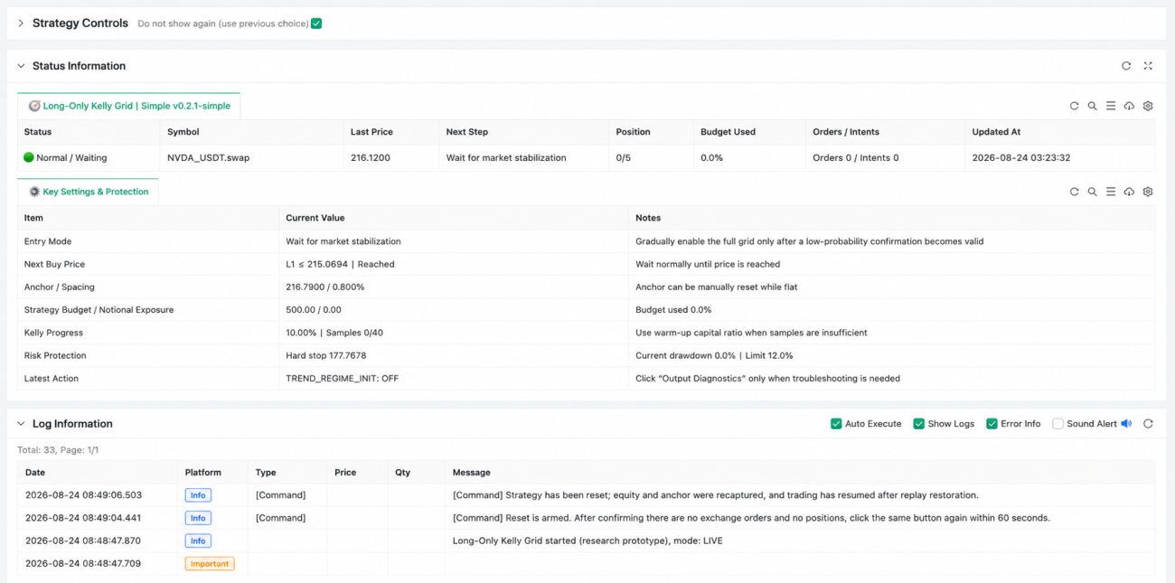
I prefer to think of Kelly in this strategy as a budget approval mechanism, not an automatic accelerator.
The grid says:
“Price has reached the second level. I want to buy again.”
The Kelly layer does not answer:
“How many times larger should the next order be?”
Instead, it asks:
How much total risk budget is currently supported by the sample? Will this action push total exposure beyond that budget?
If the sample does not support positive log growth, the answer may be zero.
If existing exposure is already above the newly estimated budget, the answer may be to reduce the position first.
Only by separating when to trade from how much total risk the strategy is allowed to take can a grid avoid automatically granting itself a larger risk budget precisely when the market is moving most strongly against it.
The next genuinely valuable step is not to add more formulas. It is to complete FMZ import validation, establish the five baseline variants, and place fees, slippage, funding costs, and out-of-sample periods into the same results table.
Only then can we answer the most important question behind this idea:
Does adding fractional Kelly to a grid strategy actually improve the trade-off between capital growth and drawdown, or does it merely make the strategy look more sophisticated?
Risk Warning: This article is intended solely for research on quantitative strategies, program design, and platform-interface discussion. It does not constitute investment advice. Perpetual contracts may involve leverage, liquidation, funding rates, liquidity risk, gap risk, tracking error, and platform technical failures. A research prototype must go through backtesting, out-of-sample validation, paper trading, and extremely small-capital testing before it can be considered for production use.
Thank you for reading and for your support.
- 1