Overview
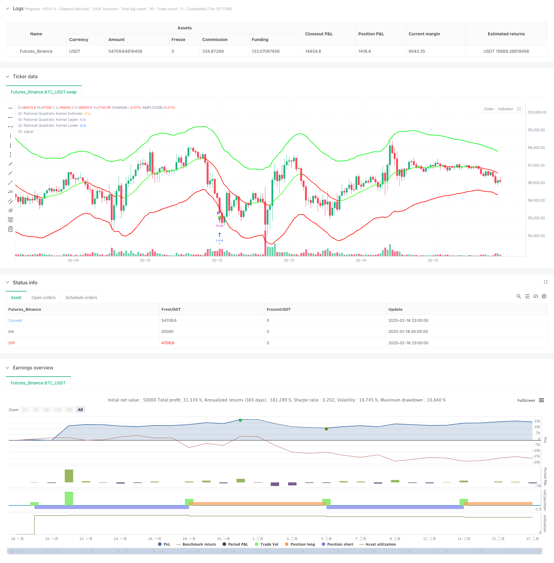
This strategy is an adaptive trend following system that combines Nadaraya-Watson kernel regression with ATR dynamic bands. It predicts price trends using rational quadratic kernel function and identifies trading opportunities through ATR-based dynamic support and resistance bands. The system achieves precise market modeling through configurable lookback window and weighting parameters.
Strategy Principle
The core of the strategy is non-parametric kernel regression based on the Nadaraya-Watson method, using a rational quadratic kernel function to smooth price series. The regression calculation starts from a specified bar, controlled by two key parameters: lookback window (h) and relative weighting ®. Dynamic bands are constructed using ATR indicator, with upper and lower bands being regression estimates plus/minus ATR multiples. Trading signals are triggered by price crossovers with the bands - long when price breaks below the lower band, short when it breaks above the upper band. Trend determination can be based on either rate of change or crossover mechanism, visualized through color changes.
Strategy Advantages
- Kernel regression has solid mathematical foundation, effectively capturing price trends without overfitting
- Dynamic bands adapt to market volatility, providing more reasonable support and resistance levels
- Strong parameter configurability, flexible adjustment for different market characteristics
- Flexible trend identification mechanism, choice between smooth or sensitive modes
- Intuitive visualization, clear trading signals
Strategy Risks
- Improper parameter selection may lead to overfitting or lag
- May generate excessive trading signals in ranging markets
- Unreasonable ATR multiplier settings can result in stop-loss being too wide or too narrow
- False signals may occur during trend transitions It is recommended to optimize parameters through historical backtesting and combine with other indicators for confirmation.
Strategy Optimization Directions
- Incorporate volume indicators for trend confirmation
- Develop adaptive parameter optimization mechanism
- Add trend strength filter to reduce false signals in ranging markets
- Optimize stop-loss and take-profit mechanism to improve risk-reward ratio
- Consider adding market environment classification to use different parameters in different markets
Summary
This strategy combines statistical learning methods with technical analysis to build a trading system with solid theoretical foundation and strong practicality. Its adaptive features and configurability enable it to adapt to different market environments, but attention needs to be paid to parameter optimization and risk control when using it. Through continuous improvement and optimization, this strategy has the potential to play an important role in practical trading.
/*backtest
start: 2025-01-18 00:00:00
end: 2025-02-17 00:00:00
period: 1h
basePeriod: 1h
exchanges: [{"eid":"Futures_Binance","currency":"BTC_USDT"}]
*/

// This source code is subject to the terms of the Mozilla Public License 2.0 at https://mozilla.org/MPL/2.0/
// © Lupown

//@version=5
strategy("Nadaraya-Watson non repainting Strategy", overlay=true)  // PARAMETER timeframe ODSTRÁNENÝ

//--------------------------------------------------------------------------------
// INPUTS
//--------------------------------------------------------------------------------
src = input.source(close, 'Source')
h   = input.float(8., 'Lookback Window', minval=3., tooltip='The number of bars used for the estimation. This is a sliding value that represents the most recent historical bars. Recommended range: 3-50')
r   = input.float(8., 'Relative Weighting', step=0.25, tooltip='Relative weighting of time frames. As this value approaches zero, the longer time frames will exert more influence on the estimation. As this value approaches infinity, the behavior of the Rational Quadratic Kernel will become identical to the Gaussian kernel. Recommended range: 0.25-25')
x_0 = input.int(25, "Start Regression at Bar", tooltip='Bar index on which to start regression. The first bars of a chart are often highly volatile, and omission of these initial bars often leads to a better overall fit. Recommended range: 5-25')
showMiddle    = input.bool(true, "Show middle band")
smoothColors  = input.bool(false, "Smooth Colors", tooltip="Uses a crossover based mechanism to determine colors. This often results in less color transitions overall.", inline='1', group='Colors')
lag           = input.int(2, "Lag", tooltip="Lag for crossover detection. Lower values result in earlier crossovers. Recommended range: 1-2", inline='1', group='Colors')

lenjeje = input.int(32, "ATR Period",    tooltip="Period to calculate upper and lower band", group='Bands')
coef    = input.float(2.7, "Multiplier", tooltip="Multiplier to calculate upper and lower band", group='Bands')

//--------------------------------------------------------------------------------
// ARRAYS & VARIABLES
//--------------------------------------------------------------------------------
float y1 = 0.0
float y2 = 0.0
srcArray = array.new<float>(0)
array.push(srcArray, src)
size = array.size(srcArray)

//--------------------------------------------------------------------------------
// KERNEL REGRESSION FUNCTIONS
//--------------------------------------------------------------------------------
kernel_regression1(_src, _size, _h) =>
    float _currentWeight = 0.
    float _cumulativeWeight = 0.
    for i = 0 to _size + x_0
        y = _src[i]
        w = math.pow(1 + (math.pow(i, 2) / ((math.pow(_h, 2) * 2 * r))), -r)
        _currentWeight    += y * w
        _cumulativeWeight += w
    [_currentWeight, _cumulativeWeight]

[currentWeight1, cumulativeWeight1] = kernel_regression1(src, size, h)
yhat1 = currentWeight1 / cumulativeWeight1

[currentWeight2, cumulativeWeight2] = kernel_regression1(src, size, h - lag)
yhat2 = currentWeight2 / cumulativeWeight2

//--------------------------------------------------------------------------------
// TREND & COLOR DETECTION
//--------------------------------------------------------------------------------
// Rate-of-change-based
bool wasBearish   = yhat1[2] > yhat1[1]
bool wasBullish   = yhat1[2] < yhat1[1]
bool isBearish    = yhat1[1] > yhat1
bool isBullish    = yhat1[1] < yhat1
bool isBearishChg = isBearish  and wasBullish
bool isBullishChg = isBullish  and wasBearish

// Crossover-based (for "smooth" color changes)
bool isBullishCross  = ta.crossover(yhat2, yhat1)
bool isBearishCross  = ta.crossunder(yhat2, yhat1)
bool isBullishSmooth = yhat2 > yhat1
bool isBearishSmooth = yhat2 < yhat1

color c_bullish    = input.color(#3AFF17, 'Bullish Color', group='Colors')
color c_bearish    = input.color(#FD1707, 'Bearish Color', group='Colors')

color colorByCross = isBullishSmooth ? c_bullish : c_bearish
color colorByRate  = isBullish       ? c_bullish : c_bearish
color plotColor    = smoothColors ? colorByCross : colorByRate

// Middle Estimate
plot(showMiddle ? yhat1 : na, "Rational Quadratic Kernel Estimate", color=plotColor, linewidth=2)

//--------------------------------------------------------------------------------
// UPPER / LOWER BANDS
//--------------------------------------------------------------------------------
upperjeje = yhat1 + coef * ta.atr(lenjeje)
lowerjeje = yhat1 - coef * ta.atr(lenjeje)

plotUpper = plot(upperjeje, "Rational Quadratic Kernel Upper", color=color.rgb(0, 247, 8), linewidth=2)
plotLower = plot(lowerjeje, "Rational Quadratic Kernel Lower", color=color.rgb(255, 0, 0), linewidth=2)

//--------------------------------------------------------------------------------
// SYMBOLS & ALERTS
//--------------------------------------------------------------------------------
plotchar(ta.crossover(close, upperjeje),  char="🥀", location=location.abovebar, size=size.tiny)
plotchar(ta.crossunder(close, lowerjeje), char="🍀", location=location.belowbar, size=size.tiny)

// Alerts for Color Changes (estimator)
alertcondition(smoothColors ? isBearishCross : isBearishChg, title="Bearish Color Change", message="Nadaraya-Watson: {{ticker}} ({{interval}}) turned Bearish ▼")
alertcondition(smoothColors ? isBullishCross : isBullishChg, title="Bullish Color Change", message="Nadaraya-Watson: {{ticker}} ({{interval}}) turned Bullish ▲")

// Alerts when price crosses upper and lower band
alertcondition(ta.crossunder(close, lowerjeje), title="Price close under lower band", message="Nadaraya-Watson: {{ticker}} ({{interval}}) crossed under lower band 🍀")
alertcondition(ta.crossover(close, upperjeje),  title="Price close above upper band", message="Nadaraya-Watson: {{ticker}} ({{interval}}) Crossed above upper band 🥀")

//--------------------------------------------------------------------------------
// STRATEGY LOGIC (EXAMPLE)
//--------------------------------------------------------------------------------
if ta.crossunder(close, lowerjeje)
    // zatvoriť short
    strategy.close("Short")
    // otvoriť long
    strategy.entry("Long", strategy.long)

if ta.crossover(close, upperjeje)
    // zatvoriť long
    strategy.close("Long")
    // otvoriť short
    strategy.entry("Short", strategy.short)