Multi-Dimensional Technical Indicator Fusion Trend Recognition Strategy

Overview

The Multi-Dimensional Technical Indicator Fusion Trend Recognition Strategy is an innovative quantitative trading approach that integrates seven different types of technical indicators to construct a robust trend identification system. The strategy employs a voting mechanism to synthesize multiple independent trend signals into a comprehensive trend judgment, thereby improving the accuracy and reliability of trend recognition. This multi-indicator fusion method effectively reduces false signals from individual indicators, providing traders with more stable and trustworthy entry timing. The strategy encompasses multiple dimensions including trend following, momentum analysis, volatility measurement, and oscillation identification, forming a comprehensive market analysis framework.

Strategy Principles

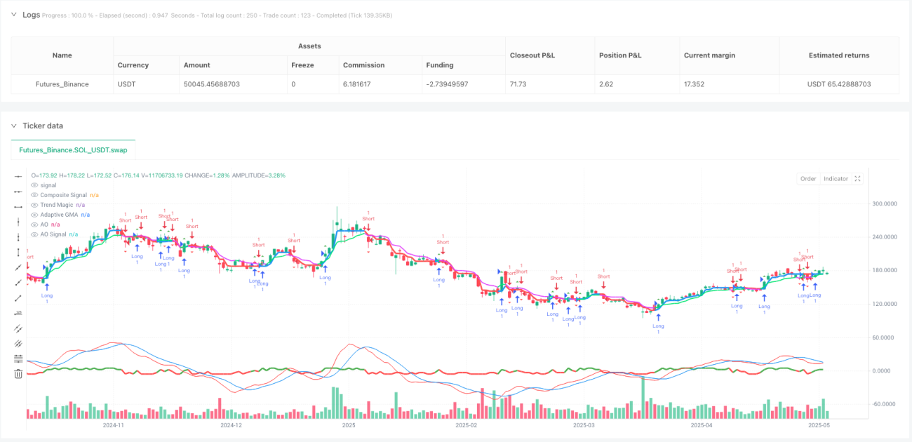
The core principle of this strategy is based on the multi-dimensional verification concept of technical analysis. First, the strategy integrates Michael’s EMA system, determining short-term trend direction by comparing fast and slow EMA sources. Second, the Trend Magic indicator combines CCI (Commodity Channel Index) and ATR (Average True Range), using CCI’s zero line as a trend judgment benchmark while employing ATR-adjusted upper and lower bands to determine dynamic support and resistance levels for trends. Third, the Adaptive GMA (Gaussian Moving Average) uses Gaussian weight distribution to calculate moving averages and can automatically adjust parameters based on market volatility, providing smoother and more sensitive trend signals. Fourth, the STC proxy indicator approximates the functionality of Stochastic Trend Channel through ROC (Rate of Change). Fifth, the WaveTrend indicator identifies wave trends based on zero-line judgment of price sources. Sixth, the traditional ROC indicator calculates price change rates over specified periods. Finally, the Awesome Oscillator determines momentum trends through the relationship between the difference of fast and slow moving averages and their signal line.

Each sub-indicator generates binary signals of +1 (bullish) or -1 (bearish), and the strategy performs simple summation of these seven signals to form a composite trend score ranging from -7 to +7. Bullish signals are triggered when the composite score transitions from non-positive to positive, while bearish signals are triggered when it transitions from non-negative to negative. This cross-detection mechanism ensures trading signals are generated only when the majority of indicators reach consensus.

Strategy Advantages

The Multi-Dimensional Technical Indicator Fusion Strategy possesses significant technical advantages. First, the multi-indicator verification mechanism dramatically reduces the probability of false signals, as misjudgments from individual indicators rarely affect overall judgment results. Second, the strategy covers different types of technical analysis methods, including trend following, momentum analysis, volatility measurement, and oscillation indicators, forming a complementary analytical system. Third, adaptive parameter design enables the strategy to automatically adjust according to changing market environments, particularly the volatility adaptation feature of the GMA indicator enhances the strategy’s environmental adaptability. Fourth, binary signal processing simplifies complex market information, making the decision-making process clearer and more definitive. Fifth, the continuity characteristics of composite signals avoid frequent signal switching, helping reduce trading costs and slippage losses. Sixth, the strategy framework has excellent scalability, allowing convenient addition or removal of indicator components. Seventh, the independent switch design for each indicator allows traders to flexibly configure indicator combinations based on market characteristics.

Strategy Risks

Despite its multiple advantages, the strategy still has potential risks that require attention. First, multi-indicator synchronization risk may cause the strategy to react sluggishly in rapidly changing markets, as it needs to wait for majority consensus among indicators before generating signals. Second, indicator redundancy risk may occur when high correlation exists between certain indicators, failing to actually add independent verification dimensions. Third, the complexity of parameter optimization grows exponentially with the number of indicators, potentially facing overfitting risks. Fourth, frequent oscillations in sideways markets may cause composite signals to repeatedly switch around the zero line, generating excessive noise trading. Fifth, the simple equal-weight summation method may lack flexibility, potentially requiring different weight allocation based on indicator reliability in certain situations.

To mitigate these risks, the following solutions are recommended: implement indicator correlation analysis to avoid redundancy; introduce signal confirmation mechanisms to reduce noise in oscillating markets; consider dynamic weight allocation to improve indicator combination effectiveness; set minimum signal strength thresholds to filter weak signals; combine market regime identification for dynamic strategy parameter adjustment.

Strategy Optimization Directions

The strategy has several important optimization directions worth deep exploration. First, an intelligent weight allocation mechanism can assign dynamic weights to different indicators based on historical performance and current market environment, rather than simple equal-weight summation. This can highlight well-performing indicators while reducing the influence of poorly performing ones. Second, market regime identification functionality can help the strategy distinguish between trending markets, oscillating markets, and transition periods, enabling the most suitable indicator combinations for different market environments. Third, signal strength grading can extend simple binary signals to multi-level signals, providing different weights based on each indicator’s signal strength to make composite signals more refined. Fourth, adaptive threshold mechanisms can dynamically adjust signal trigger thresholds based on market volatility, raising thresholds during high volatility periods to reduce noise and lowering them during low volatility periods to capture weak signals. Fifth, introducing machine learning algorithms can achieve automatic optimization of indicator combinations and dynamic parameter adjustment. Sixth, adding risk management modules including stop-loss, take-profit, and position management functions to organically combine signal generation with risk control.

Implementation of these optimization directions will significantly enhance the strategy’s practicality and profitability, enabling it to adapt to broader market environments and trading requirements.

Conclusion

The Multi-Dimensional Technical Indicator Fusion Trend Recognition Strategy represents the frontier development direction of quantitative trading technical analysis. By cleverly integrating seven different types of technical indicators, the strategy constructs a robust and comprehensive trend identification system. Its multi-indicator verification mechanism, adaptive parameter design, and modular architecture provide traders with powerful analytical tools. While the strategy faces challenges in complexity management and parameter optimization, its potential optimization space is enormous, particularly in introducing intelligent weight allocation, market regime identification, and machine learning technologies. For quantitative traders seeking stable and reliable trend signals, this multi-dimensional fusion approach provides a strategy framework worthy of deep research and practice. With continuous technological development and optimization, the strategy is expected to demonstrate excellent performance in actual trading.