Neural Network Price Differential Optimized Quantitative Trading Strategy

Overview
The Neural Network Price Differential Optimized Quantitative Trading Strategy is a high-frequency trading system based on Artificial Neural Networks (ANN), specifically optimized for 1-second timeframes. This strategy utilizes neural networks to analyze short-term price differential movements, predicts price direction through forward propagation algorithms, and combines volatility filtering and session time control to optimize trading decisions. The core of the strategy lies in capturing minute price movement patterns to achieve stable trading performance with a high profit factor (3.754) in a high-frequency environment.
Strategy Principles
The strategy employs a three-layer neural network architecture with forward propagation to process price differential data:
-
Input Layer (L0): Receives the percentage difference between the current OHLC4 (Open, High, Low, Close average) and a reference timeframe's historical OHLC4 (default 15 seconds) as a single input neuron.
-
First Hidden Layer (L1): Contains 5 neurons using hyperbolic tangent (tanh) as the activation function to perform non-linear transformation on the input data. Each neuron has pre-trained weights to capture specific patterns in price differentials.
-
Second Hidden Layer (L2): Contains 33 neurons, also using tanh activation functions, processing the first hidden layer's output through a more complex weight matrix.
-
Output Layer (L3): A single neuron outputs the final prediction signal, with its value inverted to correct signal direction.
The trading logic revolves around the neural network output value (L3_0):
- When L3_0 exceeds the entry threshold (default 0.003), a long signal is triggered
- When L3_0 falls below the negative entry threshold (-0.003), a short signal is triggered
- When L3_0 falls below the exit threshold (default 0.001), long positions are closed
- When L3_0 rises above the negative exit threshold (-0.001), short positions are closed
The strategy also implements a triple filtering mechanism:
- Cooldown Filter: After executing a trade, the system enforces a waiting period (default 60 seconds)
- Volatility Filter: Using the ATR (Average True Range) indicator, trading only occurs when market volatility exceeds a minimum threshold (default 0.02)
- Session Filter: Optionally restricting trading to specific market hours (default 9:00 to 16:00)
Strategy Advantages
-
High-Precision Predictive Capability: The multi-layer structure of the neural network can capture complex non-linear relationships in price movements that traditional technical indicators struggle to identify. Especially in high-frequency environments, this structure can recognize short-term price patterns, providing more accurate entry and exit signals.
-
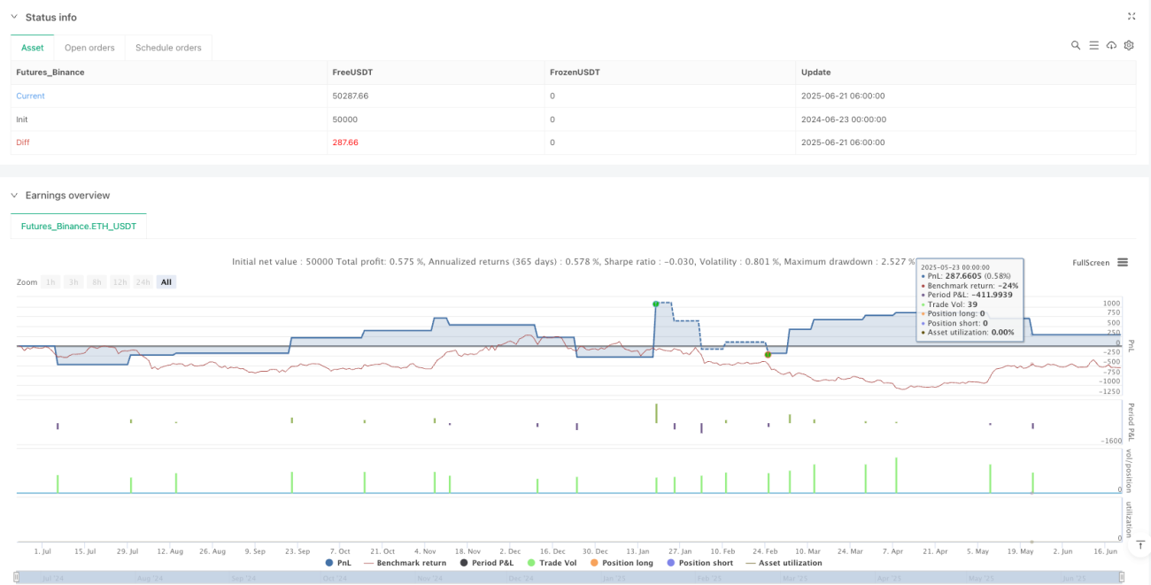
Excellent Risk-Reward Ratio: The strategy achieves a profit factor of 3.754, meaning the total of profitable trades is 3.754 times the total of losing trades, which is an outstanding performance in quantitative strategies.
-
Flexible Parameter Optimization Space: The strategy provides multiple adjustable parameters, including entry/exit thresholds, cooldown period length, reference timeframe, and minimum volatility requirements, allowing traders to optimize based on different market environments and trading instruments.
-
Multiple Filtering Mechanisms: By integrating cooldown period, volatility, and trading session triple filtering, the strategy effectively reduces unnecessary trades and false signals, improving trade quality.
-
Adaptation to High-Frequency Trading Environment: Optimized for 1-second timeframes, the strategy can fully leverage the characteristics of high-frequency trading to capture profit opportunities from short-term price fluctuations.
-
Low-Latency Implementation: The strategy code structure is clear and efficient, with the neural network portion using pre-trained weights for direct calculation, eliminating the need for real-time training and ensuring low-latency execution in high-frequency environments.
Strategy Risks
-
Overfitting Risk: The neural network model contains numerous preset weight parameters, risking overfitting to historical data. This may cause the strategy to perform worse in live trading than in backtesting, especially when market conditions change significantly. Mitigation approaches include: periodically retraining the neural network, using longer timeframe data for validation, and implementing robust risk management measures.
-
Parameter Sensitivity: Strategy performance heavily depends on multiple parameter settings, such as entry/exit thresholds and cooldown period length. Minor changes in parameters may lead to significant fluctuations in strategy performance. It is recommended to find stable parameter combinations through parameter scanning and step testing, avoiding excessive optimization.
-
High-Frequency Trading Risks: At the 1-second timeframe level, trading costs (such as spreads and slippage) can significantly impact strategy profitability. These costs should be fully considered before live trading, and realistic trading costs should be simulated in backtests.
-
Technical Implementation Challenges: High-frequency strategies require trading systems with extremely low latency and high reliability. Any network delay, data delay, or execution delay may cause strategy failure. Ensure the use of professional-grade trading infrastructure and low-latency data sources.
-
Market Volatility Risk: Under extreme market conditions (such as breaking news or liquidity drought), the neural network model may fail to accurately predict price movements, leading to substantial losses. It is advisable to set stop-loss measures and maximum daily loss limits, and to pause strategy operation during periods of extreme volatility.
Strategy Optimization Directions
-
Neural Network Architecture Optimization:
- Consider introducing more input features, such as volume, volatility indicators, and price momentum indicators, to enhance model predictive capability
- Try different hidden layer structures and neuron counts to find the optimal balance between complexity and generalization ability
- Explore the effects of other activation functions (such as ReLU or Leaky ReLU), which perform better than tanh in some neural network applications
-
Dynamic Parameter Adjustment Mechanism:
- Implement entry/exit thresholds that adaptively adjust based on market states, such as increasing thresholds in high-volatility environments and decreasing them in low-volatility environments
- Develop volatility-aware cooldown period adjustment algorithms to maintain optimal trading frequency across different market phases
-
Integrated Prediction Framework:
- Combine neural network models from multiple timeframes to form comprehensive prediction signals
- Introduce machine learning meta-models to dynamically adjust weights of different prediction models
- This approach can reduce the limitations of a single model and improve prediction stability
-
Risk Management Enhancement:
- Develop dynamic position sizing systems that adjust trading size based on model confidence and market conditions
- Introduce machine learning-based stop-loss strategies to optimize the risk-reward ratio for each trade
- Implement intraday session optimization to identify the time periods when the strategy performs best
-
Real-time Learning and Adaptation:
- Design online learning mechanisms enabling the neural network to continuously learn from new data and adapt to market changes
- Implement automatic retraining triggers based on performance monitoring, actively updating the model when strategy performance declines
- This approach can significantly improve the strategy's lifespan and stability
Summary
The Neural Network Price Differential Optimized Quantitative Trading Strategy represents cutting-edge practice in modern quantitative trading, successfully applying artificial neural network technology to high-frequency trading. Through a carefully designed multi-layer neural network structure, the strategy can capture subtle patterns in short-term price movements and improve trade quality through multiple filtering mechanisms.
The profit factor of 3.754 demonstrates the strategy's excellent performance in testing environments, but practical application still requires careful consideration of overfitting, parameter sensitivity, and risks specific to high-frequency trading. Through continuous optimization of the neural network architecture, implementation of dynamic parameter adjustments, and enhancement of risk management, this strategy has the potential to maintain long-term competitiveness in the highly competitive field of quantitative trading.
The key success factor of the strategy lies in combining complex neural network technology with practical trading logic, leveraging both the predictive capabilities of machine learning and the feasibility of actual trading. For experienced quantitative traders, this provides a scalable framework that can be further customized and optimized according to different markets and personal risk preferences.
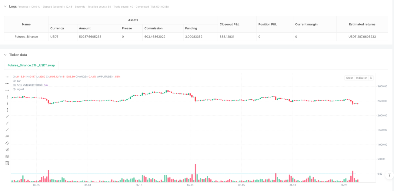
/*backtest
start: 2024-06-23 00:00:00
end: 2025-06-21 08:00:00
period: 2h
basePeriod: 2h
exchanges: [{"eid":"Futures_Binance","currency":"ETH_USDT"}]
*/

//@version=5
strategy("ANN Strategy v2 (Optimized for 1s)", overlay=true, default_qty_type=strategy.percent_of_equity, default_qty_value=100)

// === INPUTS ===- 1