Adaptive Moving Average Grid Quantitative Trading Strategy

Overview
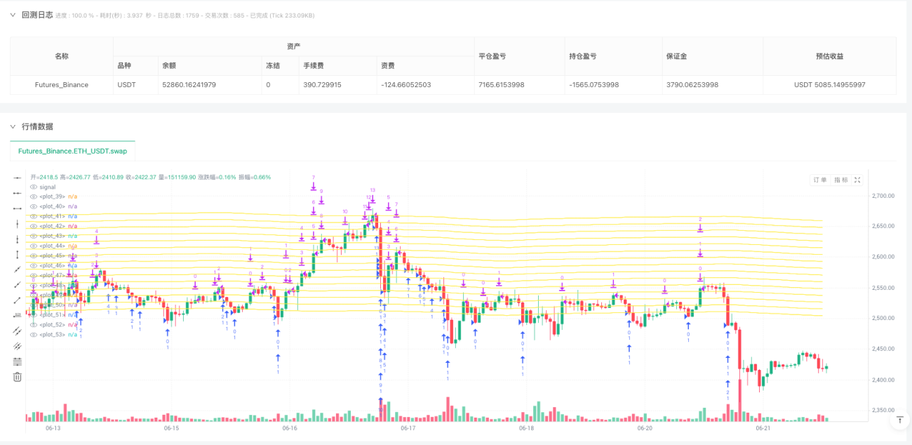
The Adaptive Moving Average Grid Quantitative Trading Strategy is a quantitative approach that combines moving average and grid trading concepts. This strategy calculates a Simple Moving Average (SMA) as the central line representing market trend, then establishes grid lines at specific percentage intervals above and below this center line. When price fluctuates between these grid lines, the strategy buys when price touches lower grid lines and sells when price touches higher grid lines. This trading method is particularly suitable for market environments where prices fluctuate within a range while generally oscillating around the moving average.
Strategy Principle
The core principle of the Adaptive Moving Average Grid Quantitative Trading Strategy is based on the mean reversion property of market prices. The strategy is implemented through the following steps:
- Calculate the Simple Moving Average (SMA) of prices as the market's middle reference value. The code uses a 300-hour moving average, a period long enough to filter short-term fluctuations.
- Set upper and lower deviation rates (3% in this example) based on the moving average to determine the upper and lower boundaries of grid trading.
- Distribute grid lines evenly between the upper and lower boundaries according to the user-defined number of grid lines (maximum 15).
- Use a boolean array to record the position status of each grid position to ensure accurate execution of trades.
- Trading logic:
- When the price falls below a grid line and no position is held at that level, buy at that grid position.
- When the price rises above a grid line and a position is held at the next lower grid position, close that lower position.
The essence of this strategy is to capture high-frequency fluctuations within a certain price range, achieving "buy low, sell high." The strategy allows holding multiple positions simultaneously (up to 15), with each position corresponding to different grid lines. This design enables the strategy to more fully utilize price fluctuations.
Strategy Advantages
The Adaptive Moving Average Grid Quantitative Trading Strategy offers the following significant advantages:
- Strong Adaptability: The strategy automatically adjusts grid positions based on moving averages, adapting to different market environments and price level changes.
- Risk Diversification: By trading across multiple grid positions, it achieves diversified capital allocation, reducing the risk of individual trades.
- Frequent Profit Opportunities: In oscillating markets, the strategy can frequently capture profit opportunities from small-amplitude fluctuations.
- Clear Entry and Exit Signals: Trading signals are based on clear conditions of price touching grid lines, reducing subjective judgment and improving consistency in strategy execution.
- Simple Parameters: The strategy requires adjusting only three main parameters: moving average length, grid deviation rate, and number of grid lines, making it easy to optimize and backtest.
- Clear Logic: Using array structures to store grid prices and order status, the code logic is clear, easy to understand and maintain.
- Visualization Support: The strategy provides visualization of grid lines, allowing traders to intuitively observe trading ranges and potential trading points.
Strategy Risks
Despite its reasonable design, the strategy still has the following potential risks:
- Trend Market Risk: In strong trending markets, prices may continue to develop in one direction, causing the strategy to continuously open positions on one side while lacking opportunities to close positions, thereby increasing capital occupation and potentially generating significant losses. The solution is to add trend filtering conditions or set maximum position limits.
- Parameter Sensitivity: The settings of moving average length and grid deviation rate have a significant impact on strategy performance. Inappropriate parameters may cause the grid to be too wide (low trading frequency) or too narrow (increased false signals). It is recommended to determine the optimal parameter combination through extensive backtesting.
- Capital Management Risk: The strategy allows up to 15 positions in the same direction, which may lead to excessive concentration of funds if the proportion of funds for each trade is not reasonably controlled. Fixed percentage of funds for each trade or dynamic adjustment of position size should be set.
- Slippage and Fee Impact: High-frequency trading strategies are more sensitive to slippage and fees, especially when the grid is narrow. It is recommended to consider these cost factors in backtesting and adjust grid width accordingly.
- Liquidity Risk: In low liquidity markets or during periods of violent fluctuations, it may be difficult to execute trades at ideal prices, affecting strategy performance. Choose trading instruments with adequate liquidity and consider setting slippage protection.
Strategy Optimization Directions
Based on the analysis of the code, the strategy can be optimized in the following directions:
- Add Trend Filters: Combine other technical indicators (such as MACD, RSI, or DMI) to determine market trends, pause or adjust grid trading strategies in obvious trending markets to avoid losses from counter-trend trading.
- Dynamic Grid Width: Dynamically adjust grid deviation rates based on market volatility (such as ATR indicator), widening grid spacing when volatility increases and narrowing grid spacing when volatility decreases, better adapting to different market conditions.
- Introduce Stop-Loss Mechanism: Set stop-loss conditions for each grid position to protect capital safety when the market experiences abnormal fluctuations. Consider dynamic stop-loss based on ATR or fixed percentage stop-loss.
- Optimize Capital Management: Implement dynamic position management, adjusting the proportion of funds for each trade based on account funds, market volatility, and existing positions, improving capital utilization efficiency and risk control capability.
- Add Time Filters: Analyze market characteristics at different time periods, activate the strategy during periods suitable for grid trading, and reduce trading frequency or pause trading during unsuitable periods.
- Multi-Timeframe Confirmation: Combine longer and shorter timeframes for trade confirmation to reduce false signals and ineffective trades.
- Optimize Code Efficiency: The grid line visualization part in the current code uses repeated plot statements, which can be optimized using loop structures to improve code conciseness and maintainability.
Summary
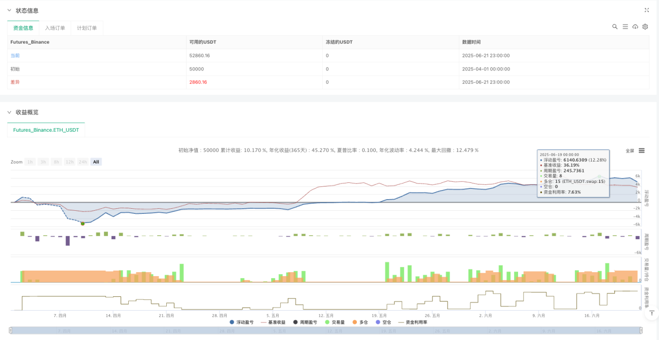
The Adaptive Moving Average Grid Quantitative Trading Strategy is a grid trading system based on the principle of mean reversion, capturing trading opportunities from price fluctuations by setting grids around moving averages. The strategy design is concise and clear, with few parameters that are easy to adjust, and is particularly suitable for application in oscillating markets. The main advantages of the strategy lie in its adaptability and risk diversification characteristics, automatically adapting to different price levels and spreading risk through multiple grid positions.
However, the strategy may face risks in strong trending markets and needs to add trend filtering and stop-loss mechanisms for optimization. In addition, dynamically adjusting grid width, improving capital management, and adding multi-timeframe confirmation are also worth exploring as optimization directions. Through these optimizations, the strategy is expected to achieve more stable and excellent performance in different market environments.
For experienced quantitative traders, this strategy provides a good foundation framework that can be further customized and optimized according to individual trading styles and risk preferences, leveraging the advantages of grid trading in capturing market volatility.
- 1