Aperçu
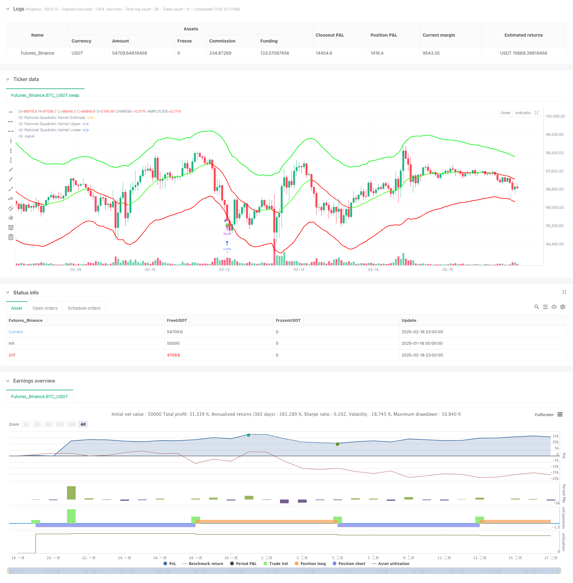
La stratégie est un système de suivi de tendance auto-adaptatif combinant la régression nucléaire de Nadaraya-Watson et la bande dynamique ATR. Il permet de prédire les tendances de prix via une fonction nucléaire rationnelle et d’identifier les opportunités de négociation en utilisant les supports et résistances dynamiques basés sur l’ATR. Le système permet une modélisation précise du marché via des fenêtres de régression et des paramètres de poids configurables.
Principe de stratégie
Le cœur de la stratégie est la régression nucléaire non paramétrique basée sur la méthode de Nadaraya-Watson, qui traite la séquence de prix de manière lisse à l’aide d’une fonction nucléaire rationnelle. La régression est calculée à partir d’une barre de départ définie, contrôlant le degré d’appariement avec les deux paramètres clés de la fenêtre de retour (lookback window ((h)) et le poids relatif (relative weight (®).
Avantages stratégiques
- La méthode de régression nucléaire a une bonne base mathématique pour capturer efficacement les tendances des prix sans surajustement
- Les bandes dynamiques s’adaptent aux fluctuations du marché et fournissent des points de résistance de soutien plus raisonnables
- Les paramètres sont configurables et peuvent être ajustés en fonction des caractéristiques du marché
- Les mécanismes de détection des tendances sont flexibles et peuvent choisir un mode lisse ou sensible.
- Les effets visuels sont intuitifs et les signaux de transaction sont clairs.
Risque stratégique
- Une mauvaise sélection de paramètres peut entraîner une suradaptation ou un retard
- Les signaux d’excès de trading peuvent être générés dans un marché en crise
- Une configuration déraisonnable du multiplicateur ATR peut entraîner un arrêt trop large ou trop étroit
- La période de transition de la tendance peut donner de faux signaux Il est recommandé d’optimiser les paramètres en utilisant la rétroaction historique et d’utiliser d’autres indicateurs comme confirmation auxiliaire.
Orientation de l’optimisation de la stratégie
- L’introduction de l’indicateur de quantité d’échange comme confirmation de tendance
- Développement de mécanismes d’optimisation des paramètres d’adaptation
- Augmentation de l’intensité de la tendance et réduction des faux signaux sur les marchés oscillants
- Optimisation du mécanisme d’arrêt des pertes pour améliorer la rentabilité
- Considérer l’ajout d’une classification des environnements de marché, avec des paramètres différents selon les marchés
Résumer
La stratégie, en combinant des méthodes d’apprentissage statistique avec l’analyse technique, construit un système de négociation solide en théorie et pratique. Ses caractéristiques d’adaptation et de configuration lui permettent de s’adapter à différents environnements de marché, mais son utilisation nécessite une attention particulière à l’optimisation des paramètres et à la maîtrise des risques.
/*backtest
start: 2025-01-18 00:00:00
end: 2025-02-17 00:00:00
period: 1h
basePeriod: 1h
exchanges: [{"eid":"Futures_Binance","currency":"BTC_USDT"}]
*/

// This source code is subject to the terms of the Mozilla Public License 2.0 at https://mozilla.org/MPL/2.0/
// © Lupown

//@version=5
strategy("Nadaraya-Watson non repainting Strategy", overlay=true)  // PARAMETER timeframe ODSTRÁNENÝ

//--------------------------------------------------------------------------------
// INPUTS
//--------------------------------------------------------------------------------
src = input.source(close, 'Source')
h   = input.float(8., 'Lookback Window', minval=3., tooltip='The number of bars used for the estimation. This is a sliding value that represents the most recent historical bars. Recommended range: 3-50')
r   = input.float(8., 'Relative Weighting', step=0.25, tooltip='Relative weighting of time frames. As this value approaches zero, the longer time frames will exert more influence on the estimation. As this value approaches infinity, the behavior of the Rational Quadratic Kernel will become identical to the Gaussian kernel. Recommended range: 0.25-25')
x_0 = input.int(25, "Start Regression at Bar", tooltip='Bar index on which to start regression. The first bars of a chart are often highly volatile, and omission of these initial bars often leads to a better overall fit. Recommended range: 5-25')
showMiddle    = input.bool(true, "Show middle band")
smoothColors  = input.bool(false, "Smooth Colors", tooltip="Uses a crossover based mechanism to determine colors. This often results in less color transitions overall.", inline='1', group='Colors')
lag           = input.int(2, "Lag", tooltip="Lag for crossover detection. Lower values result in earlier crossovers. Recommended range: 1-2", inline='1', group='Colors')

lenjeje = input.int(32, "ATR Period",    tooltip="Period to calculate upper and lower band", group='Bands')
coef    = input.float(2.7, "Multiplier", tooltip="Multiplier to calculate upper and lower band", group='Bands')

//--------------------------------------------------------------------------------
// ARRAYS & VARIABLES
//--------------------------------------------------------------------------------
float y1 = 0.0
float y2 = 0.0
srcArray = array.new<float>(0)
array.push(srcArray, src)
size = array.size(srcArray)

//--------------------------------------------------------------------------------
// KERNEL REGRESSION FUNCTIONS
//--------------------------------------------------------------------------------
kernel_regression1(_src, _size, _h) =>
    float _currentWeight = 0.
    float _cumulativeWeight = 0.
    for i = 0 to _size + x_0
        y = _src[i]
        w = math.pow(1 + (math.pow(i, 2) / ((math.pow(_h, 2) * 2 * r))), -r)
        _currentWeight    += y * w
        _cumulativeWeight += w
    [_currentWeight, _cumulativeWeight]

[currentWeight1, cumulativeWeight1] = kernel_regression1(src, size, h)
yhat1 = currentWeight1 / cumulativeWeight1

[currentWeight2, cumulativeWeight2] = kernel_regression1(src, size, h - lag)
yhat2 = currentWeight2 / cumulativeWeight2

//--------------------------------------------------------------------------------
// TREND & COLOR DETECTION
//--------------------------------------------------------------------------------
// Rate-of-change-based
bool wasBearish   = yhat1[2] > yhat1[1]
bool wasBullish   = yhat1[2] < yhat1[1]
bool isBearish    = yhat1[1] > yhat1
bool isBullish    = yhat1[1] < yhat1
bool isBearishChg = isBearish  and wasBullish
bool isBullishChg = isBullish  and wasBearish

// Crossover-based (for "smooth" color changes)
bool isBullishCross  = ta.crossover(yhat2, yhat1)
bool isBearishCross  = ta.crossunder(yhat2, yhat1)
bool isBullishSmooth = yhat2 > yhat1
bool isBearishSmooth = yhat2 < yhat1

color c_bullish    = input.color(#3AFF17, 'Bullish Color', group='Colors')
color c_bearish    = input.color(#FD1707, 'Bearish Color', group='Colors')

color colorByCross = isBullishSmooth ? c_bullish : c_bearish
color colorByRate  = isBullish       ? c_bullish : c_bearish
color plotColor    = smoothColors ? colorByCross : colorByRate

// Middle Estimate
plot(showMiddle ? yhat1 : na, "Rational Quadratic Kernel Estimate", color=plotColor, linewidth=2)

//--------------------------------------------------------------------------------
// UPPER / LOWER BANDS
//--------------------------------------------------------------------------------
upperjeje = yhat1 + coef * ta.atr(lenjeje)
lowerjeje = yhat1 - coef * ta.atr(lenjeje)

plotUpper = plot(upperjeje, "Rational Quadratic Kernel Upper", color=color.rgb(0, 247, 8), linewidth=2)
plotLower = plot(lowerjeje, "Rational Quadratic Kernel Lower", color=color.rgb(255, 0, 0), linewidth=2)

//--------------------------------------------------------------------------------
// SYMBOLS & ALERTS
//--------------------------------------------------------------------------------
plotchar(ta.crossover(close, upperjeje),  char="🥀", location=location.abovebar, size=size.tiny)
plotchar(ta.crossunder(close, lowerjeje), char="🍀", location=location.belowbar, size=size.tiny)

// Alerts for Color Changes (estimator)
alertcondition(smoothColors ? isBearishCross : isBearishChg, title="Bearish Color Change", message="Nadaraya-Watson: {{ticker}} ({{interval}}) turned Bearish ▼")
alertcondition(smoothColors ? isBullishCross : isBullishChg, title="Bullish Color Change", message="Nadaraya-Watson: {{ticker}} ({{interval}}) turned Bullish ▲")

// Alerts when price crosses upper and lower band
alertcondition(ta.crossunder(close, lowerjeje), title="Price close under lower band", message="Nadaraya-Watson: {{ticker}} ({{interval}}) crossed under lower band 🍀")
alertcondition(ta.crossover(close, upperjeje),  title="Price close above upper band", message="Nadaraya-Watson: {{ticker}} ({{interval}}) Crossed above upper band 🥀")

//--------------------------------------------------------------------------------
// STRATEGY LOGIC (EXAMPLE)
//--------------------------------------------------------------------------------
if ta.crossunder(close, lowerjeje)
    // zatvoriť short
    strategy.close("Short")
    // otvoriť long
    strategy.entry("Long", strategy.long)

if ta.crossover(close, upperjeje)
    // zatvoriť long
    strategy.close("Long")
    // otvoriť short
    strategy.entry("Short", strategy.short)