【Neutral-Hedge Statistical Arbitrage New】(Pure-Alpha dream version)

【Neutral Hedge Stat Arbitrage New】(Pure-Alpha Dream Edition)

-A robust arbitrage strategy with 0 long and short exposures

Hello all traders, after several months of debugging, optimization and iteration, I am very happy that this neutral hedging statistical arbitrage has reached a more stable level and can be seen with you. This is a market-neutral strategy based on long-short hedging. If you go long on a basket of varieties and short on a basket of varieties in the same account, the long and short values are equal. On the premise of avoiding beta systemic risks in the market, statistical methods are used to find various long-short matching combinations to achieve a low-risk arbitrage strategy of alpha stable profitability. This strategy has good holding experience, low correlation with the market, neutral long and short exposure, and no risk under extreme black swans such as 312/519. Instead, it will flourish at such a time when market pricing errors are completely chaotic. Brilliant. This strategy will be explained in detail below.

Hello~Welcome come to my channel!

Welcome all traders to my channel. I am a Quant Developer, and I develop full-stack CTA & HFT & Arbitrage and other trading strategies. Thanks to the FMZ platform, I will share more content related to quantitative development in my quantitative channel, and work with all traders to maintain the prosperity of the quantitative community.

For more information, please move to my channel~ I’m waiting for you here to tease 【TradeMan Home】

1. Introduction and explanation of statistical arbitrage

Statistical arbitrage strategy is a strategy that exploits the price relationship between different basket varieties for trading. This strategy is based on statistical principles, by analyzing the historical price trends and correlations between two or more varieties, finding the price differences between them, and using these differences for trading. Historically, cross-species pairing statistical arbitrage strategies have been widely used in the stock market. The earliest cross-species arbitrage strategies were mainly conducted between stocks in the same industry or related industries, such as oil companies or telecommunications companies. These strategies are often based on the assumption of industry correlation and achieve the purpose of arbitrage by buying undervalued stocks and selling overvalued stocks.

With the development of the market, cross-species matching statistical arbitrage strategies have gradually expanded to other financial markets, such as commodity futures, foreign exchange, and cryptocurrency. In these markets, different basket combinations can be found that are correlated and arbitrage trades can be made using price differences. The logic of this strategy is based on the principle of mean reversion. When the prices among the constructed multiple basket combinations deviate from their statistical scope, there is a regression trend. According to this trend, when the price deviates greatly, you can sell a basket of high-priced varieties and buy a basket of low-priced varieties in order to hedge against the short-term mispricing of the market. In this way, profits can be obtained from the spread of a multi-basket paired combination.

2. Advantages and Disadvantages of Statistical Arbitrage

advantage:

• Reduce market risk: Statistical arbitrage strategy is based on arbitrage transactions based on the differences between various basket product combinations. Compared with single product transactions, it disperses risks and reduces the impact of market fluctuations on the strategy. Reduce market systemic risks.
• Stable income: Statistical arbitrage strategies conduct regression arbitrage transactions against short-term market mispricings. Compared with directional strategies, they have more stable income characteristics. Compared with directional strategies, it produces lower risk, lower volatility, and stable returns.
• Can adapt to different market environments: Statistical arbitrage strategies can operate in different market environments because this trading strategy has less directional relationship with the market.

shortcoming:

• Historical data can only reflect past relationships and cannot fully represent the future, so there are certain risks. The construction of statistical arbitrage strategies will use a large number of statistical tests to mine the combinations and correlations of basket varieties based on historical big data. Changes may occur in the future and require certain risk control measures.
• It is difficult to accurately judge the time span required to return to the equilibrium relationship due to short-term pricing errors in the market. If the transaction time is too long, the cost of using funds will also be very high.
• Highly demanding data analysis and model building capabilities: Statistical arbitrage strategies require in-depth analysis and modeling of statistical data such as correlation and cointegration between different basket combinations, and require high data analysis and model building capabilities. .
• Transaction execution and liquidity risk: Since it is a cross-variety transaction, the execution price and trading volume may be affected by different varieties, and there is a transaction execution risk. More sophisticated strategy design and architecture implementation are needed.

3. The main content of this Alpha statistical arbitrage

**1, monitor all varieties of data information in real time, conduct big data scanning, and build a basket combination of long and short varieties. **

Specifically, a basket combination will be constructed: for example, if there are 6 varieties A, B, C, D, E, and F, they can be divided into 2 groups of 3 varieties each to construct a basket combination. At the same time, index arbitrage will be constructed: dividing some industries and sector varieties into two, constructing two new market indexes, and then conducting subsequent statistical data analysis on these two indexes.

**2, test the correlation of long and short basket combinations. **

Correlation refers to the degree of association between two or more variables. It is used to measure the relationship between changes in one variable and changes in another variable, helping to determine whether there is a certain correspondence or predict the impact of changes in one variable on another variable. Correlation coefficient is a common method to measure correlation. Common ones include Pearson correlation coefficient, Spearman’s rank correlation coefficient, etc. The Pearson correlation coefficient evaluates the relationship between two continuous variables, while the Spearman rank correlation coefficient is suitable for evaluating the relationship between two ordinal variables.

The value range of the correlation coefficient is [-1, 1], where -1 indicates negative correlation, 1 indicates positive correlation, and 0 indicates no correlation. The closer the correlation coefficient is to -1 or 1, the stronger the correlation; the closer to 0, the weaker the correlation. The mathematical formula of the correlation coefficient is as follows (taking the Pearson correlation coefficient as an example):

r = cov(X, Y) / (std(X) * std(Y)).

Among them, r is the correlation coefficient, cov is the covariance, std is the standard deviation, and X and Y represent two variables respectively. When testing correlation, a common approach is to calculate the statistical significance of the correlation coefficient. Hypothesis testing can usually be used to determine whether the correlation coefficient is significant. The null hypothesis of hypothesis testing is that there is no correlation between variables, and the statistic of the correlation coefficient is calculated to determine whether to reject the null hypothesis.

**3, test the cointegration of the long-short basket combination. **

Cointegration refers to the long-term relationship between two or more time series variables, that is, their linear combination is stable. Compared with correlation, cointegration pays more attention to the long-term equilibrium relationship rather than just the short-term degree of correlation. When they deviate from this equilibrium relationship, there is a correction mechanism to return the deviation to a reasonable range. The concept of cointegration was originally proposed by Spiegelman (S.G. Engle) and C.W.J. Granger (C.W.J. Granger) in 1987 to solve the spurious regression problem existing in time series analysis. The pseudo regression problem is caused by the possible existence of unit roots between variables. The unit root makes the regression relationship between variables seem significant in the short term, but there is no real equilibrium relationship in the long term.

Cointegration theory starts from analyzing the non-stationarity of time series and explores the long-term equilibrium relationship contained in non-stationary variables. If the variables involved are stationary after first differences, and a certain linear combination of these variables is stationary, then cointegration is said to exist between these variables. Cointegration is used to describe the stationary relationship between two or more series. For each sequence individually, it may be non-stationary. The moments of these sequences, such as the mean, variance or covariance, change with time, while the linear combination sequence of these time series may have properties that do not change with time. When the prices of two assets obey the cointegration relationship, then their linear combination satisfies the property of mean reverting. The mathematical formula of cointegration is expressed as follows (taking two time series variables as an example):

Y_t = β_0 + β_1 * X_t + ε_t

Among them, Y_t and X_t represent the observed values of two time series variables respectively, β_1 is the regression coefficient, and ε_t is the error term. If there is a cointegration relationship between Y_t and X_t, then the linear combination of the two variables will be stable, that is, ε_t is stationary. Satisfies the normal distribution with mean 0. When testing cointegration, stability testing is usually required. Commonly used methods include the Johansen test and the Engle-Granger test. The Johansen test is a method based on eigenvalue, which can directly test the cointegration relationship between multiple variables. The Engle-Granger two-step test is a method based on modified OLS estimation (Ordinary Least Squares) and is suitable for testing the cointegration relationship between two variables.

**4. This strategy will test the cointegration relationship of time series for a large number of combinations. The specific standards are as follows: **

• The time price series of a separate combined basket is a first-order integral vector, that is, the time price series is non-stationary (has an obvious trend). Use the ADF unit root to test the stationarity of multiple time price times.
• The series (i.e. the derivative) after the first difference of the individual combined baskets is stationary. Use ADF unit root to test two basket time price series. Use the ADF unit root to test the stationarity of the first difference of the time price series of the two baskets.
• A certain linear combination of paired combination time price series is stationary, that is, the residual of a linear equation constructed from two series is stationary. For two sequences of the same order, perform OLS regression and then test the stationarity of the residuals.

**5, conduct a large number of Hurst index tests. **

The Hurst index is used to measure the long-term memory of a time series to determine the mean reversion properties of the series. The Hurst index value is between 0 and 1, with values close to 0.5 indicating that the sequence exhibits a random walk, and values close to 1 indicating a sustained trend. Principle: The Hurst index estimates the degree of long-term memory of a sequence by calculating the relationship between the dispersion range of overlapping subsequences of a sequence and its length. Mathematical formula: One way to calculate the Hurst index is to use the relationship between the dispersion range and length of overlapping subsequences to establish the corresponding relationship of random walks. The Hurst index can be estimated using a linear regression fit between the dispersion range and length of overlapping subsequences.

**6, mean reversion half-life estimate. **

Mean reversion half-life is a metric used to estimate the time it takes for a price series to return to its mean. The smaller the half-life, the faster the mean reversion. Principle: The calculation of the mean reversion half-life is estimated by fitting a convergent exponential smoothing moving average model (EMA). When the price series deviates from the mean by more than half-life, it can be considered that there is an opportunity for mean reversion. Mathematical formula: The calculation formula of mean reversion half-life is as follows:

(H = -\frac{\ln(0.5)}{\ln(\frac{P_t}{P_t - P_{t-1}})})

Test method: You can calculate the EMA of the price series, and then calculate the half-life based on the EMA.

**7. Construct a trading strategy based on a large amount of statistical data. **

Filter basket product combinations based on Hurst index sorting, estimate relevant parameters based on mean reversion half-life, and construct a trading strategy combination based on statistical cointegration. Suppose x and y are the price time series of the asset The normal distribution of .

After cointegration testing, it is found that there is a cointegration relationship between the time prices of assets X and Y. The standard deviation of the residual term c is σ, and the constant λ is selected as the boundary value.

• When lny-(a+blnx) > λσ, the price of basket Y is relatively overvalued and the price of basket X is relatively undervalued. Buy basket X and sell basket Y;
• When lny-(a+blnx) < -λσ, the price of basket X is relatively overvalued and the price of basket Y is relatively undervalued. Buy basket Y and sell basket X;
• When the price difference lny-(a+blnx) returns to a certain range, such as the [-0.5λσ, 0.5λσ] range, the position is closed;

**8, more to come. **

More exclusive and innovative logic, more detailed architecture and detail processing are its unique core competitiveness. At present, liquidity will be statistically estimated and transactions will be completed using market prices. In the future, it will gradually be iteratively upgraded to high-frequency statistical arbitrage of the pending order type. We look forward to paying attention and growing together.

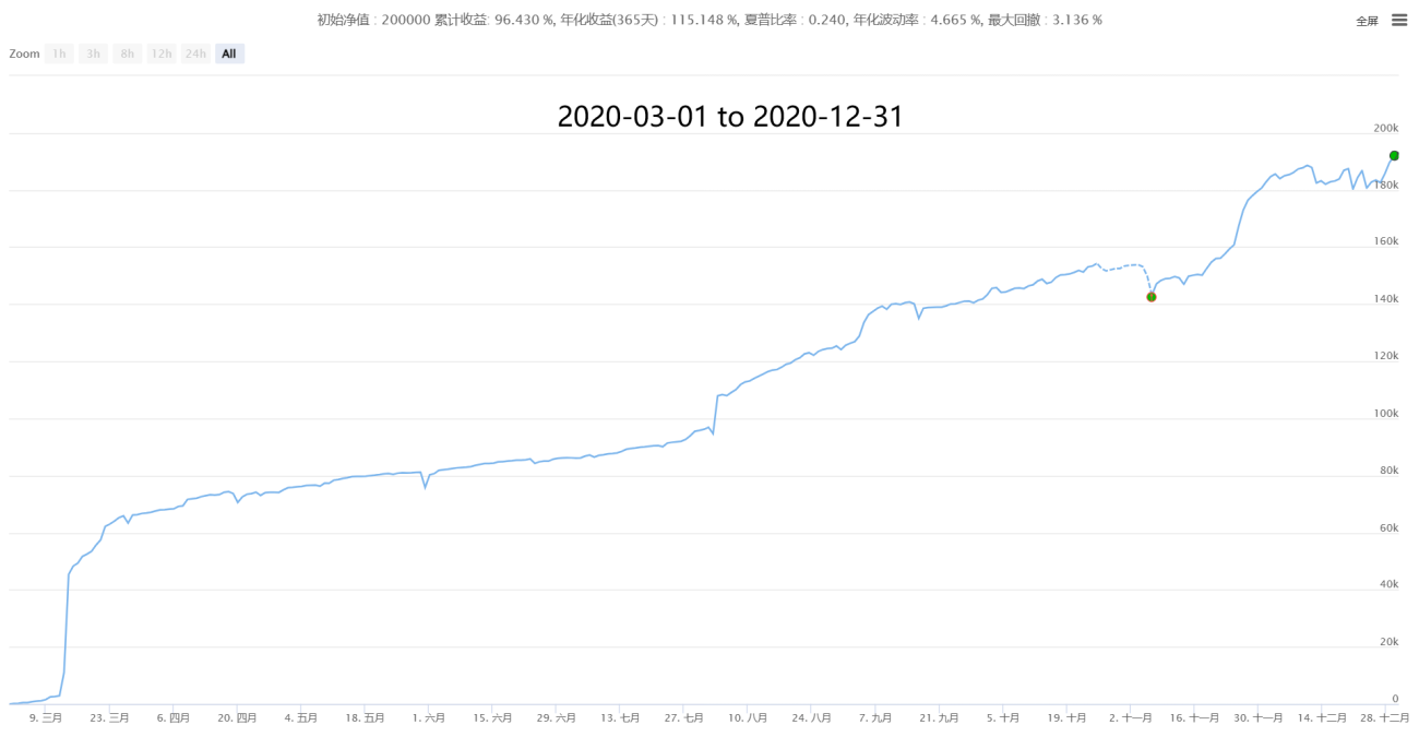
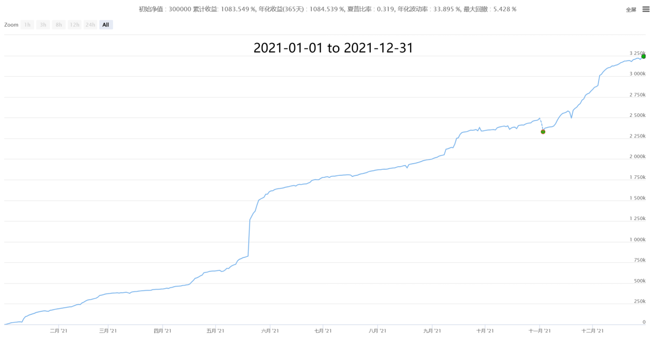
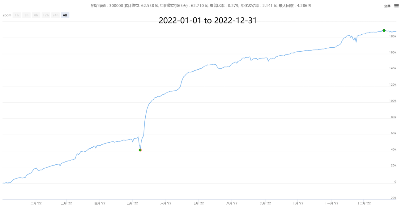
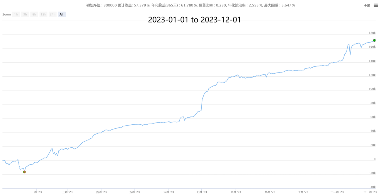
4. Partial historical performance (cost data of 50,000 orders after estimating the real transaction price)

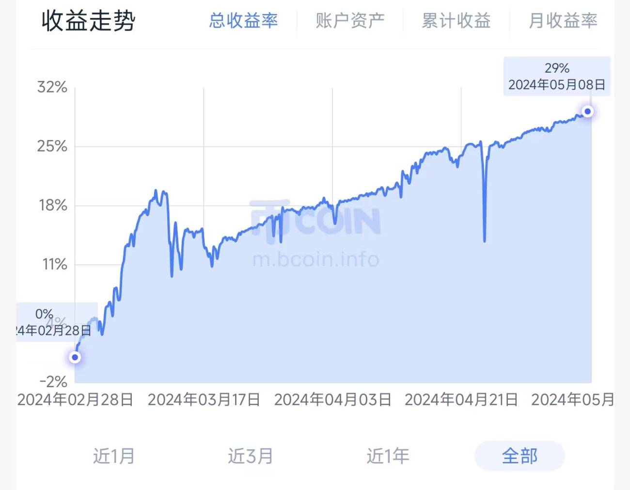
【Neutral Hedging Statistical Arbitrage New】-High-Risk Supernova 【Neutral Hedging Statistical Arbitrage New】-Low Risk and Steady

5. Looking forward to cooperation, exchanges, and joint learning and progress

Any strategy has its own methodology and suitability. For example, the mean reversion strategy is based on market random walk and other theories, and the momentum trend strategy is based on various behavioral finance theories, such as fat tail fluctuations in the market. We must understand its principles, adapt to its fluctuations based on its characteristics. At the same time, users of strategies must pay attention to the same source of profits and losses. Higher returns must be accompanied by higher risks. Mature strategies have their advantages and disadvantages. They must use them reasonably and maximize their strengths and avoid weaknesses. Know whether they are right or wrong, and whether they are appropriate or not according to the market situation. Complete performance, be confident and not be surprised.

Quantification is not a perpetual motion machine, nor is it omnipotent, but it must be the direction of future trading and is worth learning and using by every trader! Traders are welcome to come and point out shortcomings, discuss together, learn and make progress together, ride the wind and waves in the magnificent market, and forge ahead.

● Rental plan: XXXU/XU/month, the current preferential period is free for rent, and may be terminated at any time.

● Sharing plan: Large amounts can be started for free, and 20% of profits will be extracted on a monthly basis. If there is no profit, no profit will be shared.

●Strategic Commitment: If the user generates profits at the end of the lease period and does not cover the cost (the configuration and parameters are correct, and it is not a force majeure black swan), one month will be given unconditionally until profits are made.

● More cooperation options: for any individuals and institutions in need.We all maintain an open and win-win attitude towards cooperation and look forward to your discussions and customized cooperation based on your needs, risk preferences, etc.

If you have a higher risk appetite, like short-term profits and losses, and have short-term trading needs, you can check out another stable high-frequency strategy with a monthly return of 3%-50% and no risk of liquidation: 【High Frequency Hedging Market Making Grid New】(HFT Market-Making Mining Machine Version)

**If you have a large amount of funds, you can observe another large-capacity mid-low-frequency composite CTA trading system, which lasts for 900 days of real trading, rain or shine. It is the CTA strategy combination system with the longest history, high stability and strong universality currently announced to achieve medium and long-term stable growth: ** 【Compound CTA Trading System New】(Multi-factor + multi-variety + multi-strategy public version)

✱ Contact information (welcome to communicate and discuss, learn and progress together) WECHAT: haiyanyydss Telegram: https://t.me/JadeRabbitcm More useful information ➔ TradeMan Home: https://www.fmz.com/market-offer/512 ✱Fully automatic CTA & HFT & Arbitrage trading system @2018 - 2024

More