Quantitative Handelsstrategie unter Verwendung mehrerer Indikatoren zur Identifizierung von Wendepunkten im Handel

Überblick
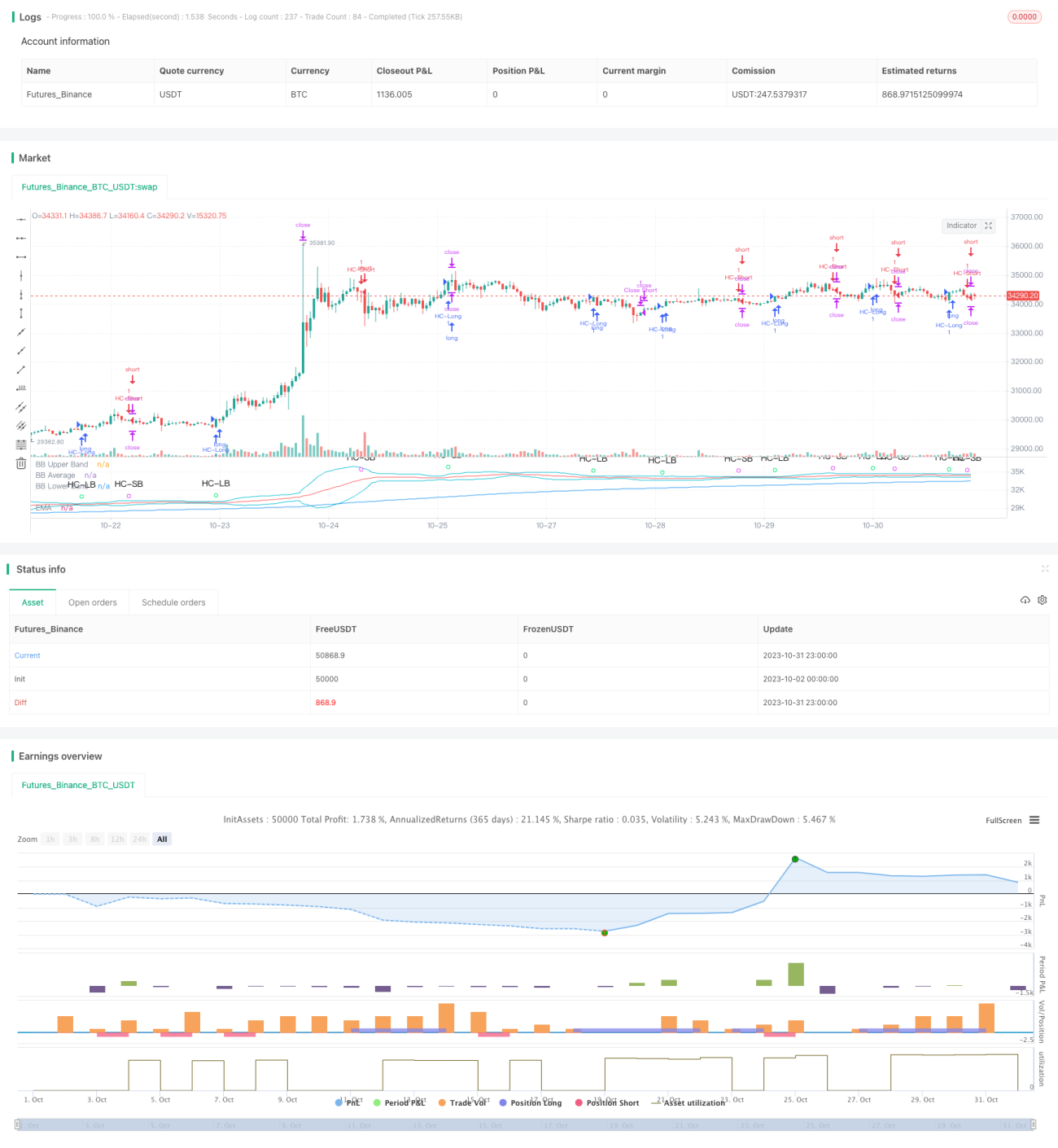
Die Strategie verwendet die fünf wichtigsten Indikatoren EMA, VWAP, MACD, Bollinger Bands und Schaff Trend Cycle zur Identifizierung von Preisumkehrpunkten in einer bestimmten Bandbreite und sendet Kauf- und Verkaufssignale aus. Der Vorteil der Strategie besteht darin, dass die Kombination anhand verschiedener Marktindikatoren angepasst werden kann, um die Wahrscheinlichkeit von Falschsignalen zu verringern und die Gewinnwahrscheinlichkeit zu erhöhen.
Strategieprinzip
-
Die EMA-Gewinnlinie beurteilt die Richtung des großen Trends und kauft nur in der Richtung des Trends
-
VWAP-Bewertung: Die Einrichtung kauft nur, wenn sie Geld bekommt
-
Die MACD beurteilt die kurze Linie Trends und Dynamikveränderungen, die MACD-Linien brechen die Signallinie als Kauf/Verkauf Signal
-
Bollinger Bands beurteilen, ob ein Über- oder Überverkauf vorliegt, wobei ein Kursübergang als Kauf-/Verkaufssignal angesehen wird.
-
Schaff Trend Cycle beurteilt die kurzfristige Kurvenumkehrstruktur und betrachtet die Überschreitung der hohen und niedrigen Schwellen als Kauf-/Verkaufssignal
-
Wenn die fünf wichtigsten Indikatoren ein einheitliches Signal senden, gibt es einen Kauf-/Verkaufsbefehl
-
Setzen Sie Stop-Loss- und Stop-Stop-Punkte und optimieren Sie die Geldverwaltung
Strategische Vorteile
- Mehrfache Kombinationen reduzieren die Wahrscheinlichkeit von Falschsignalen
Die Kombination von mehreren Indikatoren wie EMA, VWAP, MACD, BB und STC kann gegenseitig verifiziert werden, wodurch die Falschsignale, die von einem einzelnen Indikator erzeugt werden, reduziert und somit die Zuverlässigkeit des Signals erhöht wird.
- Benchmarks können angepasst werden
Die Wahl, ob ein bestimmter Indikator verwendet werden soll, kann in Kombination mit anderen Indikatoren für verschiedene Sorten und Marktumgebungen erfolgen, um die Strategie zielgerichteter und anpassungsfähiger zu machen.
- Optimierung der Geldverwaltung
Die Einrichtung von Stop-Loss- und Stop-Stop-Punkten ermöglicht die Begrenzung von Einzelschäden und die Sperrung eines Teils der Gewinne für eine bessere Verwaltung des Geldes.
- Strategie ist klar
Mit einfachen, intuitiven Kennzahlen und detaillierten Code-Kommentaren ist die gesamte Strategie so einfach zu verstehen und zu ändern, dass sie auf den ersten Blick erkennbar ist.
- Die Praxis
Die Verwendung von mehreren Indikatoren ist weit verbreitet, die Parameter sind vernünftig eingestellt, können direkt für den Handel auf der Plattform verwendet werden und können ohne große Optimierung gute Ergebnisse erzielen.
Strategisches Risiko
- Risiken bei der Identifizierung von Veränderungen nach dem Verzögerungsszenario
Indikatoren wie EMA, MACD und andere haben eine gewisse Verzögerung bei der Identifizierung von Preisänderungen und können den besten Kaufzeitpunkt verpassen.
- Gefahr, dass die Parameter falsch eingestellt sind
Wenn die Indikatorparameter nicht korrekt eingestellt sind, werden viele falsche Signale erzeugt, die die Strategie nicht funktionieren lassen.
- Die Gefahr, dass die Gewinnquote nicht garantiert ist
Eine Kombination aus mehreren Indikatoren kann die Gewinnquote erhöhen, aber nicht garantieren, dass jeder Handel gewinnt. Veränderungen der Marktumgebung können zu einer Verringerung der Gewinnquote führen.
- Der Stop-Loss-Punkt setzt ein zu kleines Risiko ein
Wenn die Stop-Loss-Punkt-Einstellung zu klein ist, kann die Stop-Loss-Ausgabe bei normalen Preisfluktuationen erfolgen, was zu unnötigen Verlusten führt.
Richtung der Strategieoptimierung
- Erhöhung der Zuverlässigkeit von Signalen durch Maschinelles Lernen
Modelle können trainiert werden, um die Zuverlässigkeit von Multi-Indikator-Signalen zu beurteilen, sie zu bewerten und Falschsignale zu reduzieren.
- Erhöhung der Quantifizierung von Indikatoren zur Identifizierung von Trends
Hinzu kommen quantitative Indikatoren wie OBV, die Anzeichen von Preissteigerungen erkennen und die Kaufsicherheit erhöhen.
- Optimierung der Stop-Loss-Strategie
Es können mobile Stop-Loss- oder Lock-In-Strategien erforscht werden, die besser für diese Strategie geeignet sind, um die Kapitalverwaltung zu optimieren.
- Parameteroptimierung
Die Optimierung der Parameter für jeden Indikator durch systematischere Rückmeldung verbessert die Gesamtstabilität der Strategie.
- Erhöhung des Robotertrags
Die Anbindung an die Transaktions-API ermöglicht automatische Bestellungen, so dass die Strategie wirklich unbemannt funktioniert.
Zusammenfassen
Diese Strategie integriert die Vorteile verschiedener technischer Indikatoren, ist klar und praktisch, kann als Entscheidungsreferenz für diskretionären Handel verwendet werden, kann aber auch direkt für algorithmischen Handel verwendet werden. Es ist jedoch erforderlich, die Anpassung an die spezifischen Sorten und die Marktumgebung zu optimieren, um das Risiko zu senken und die Stabilität zu verbessern, um letztendlich stabile Gewinne im realen Markt zu erzielen.
/*backtest
start: 2023-10-02 00:00:00
end: 2023-11-01 00:00:00
period: 1h
basePeriod: 15m
exchanges: [{"eid":"Futures_Binance","currency":"BTC_USDT"}]
*/

//@version=4

// This source code is subject to the terms of the Mozilla Public License 2.0 at https://mozilla.org/MPL/2.0/
// © MakeMoneyCoESTB2020- 1