The least common multiple of the linear regression theorem

The least common multiple of the linear regression theorem

• One, the introduction

  During this time, I learned the logistic regression algorithm in Chapter 5, which was quite challenging. I traced the origin of the algorithm from logistic regression to linear regression, and then to the logical minimum binary algorithm. I finally settled on the logical minimum binary algorithm in Chapter 9, Section 10, which explains where the mathematical principles behind the minimal binary algorithm come from. The logarithmic least squares logarithm is an implementation of the empirical formula in optimization problems. Understanding how it works is useful for understanding the logarithmic regression logarithm and the logarithmic support vector machine learning logarithms.

• Second, background knowledge

  The historical background to the appearance of the smallest two-fold square is interesting.

  In 1801, the Italian astronomer Giuseppe Piazzi discovered the first asteroid, the constellation Orion. After 40 days of tracking, Piazzi lost its position due to the constellation running behind the Sun. Subsequently, scientists around the world began searching for Orion using Piazzi's observations, but no results were found based on most people's calculations.

  Gauss's method for the least squares was published in 1809 in his Theory of Motion of the Cosmos, and the French scientist Le Jeandard independently discovered the least squares in 1806, but this was not known at the time. There was a dispute over who first established the principle of the least squares.

  In 1829, Gauss provided a proof that the optimization effect of the minimal binomial is stronger than other methods, see Gauss-Markov theorem.

• Third, use knowledge.

  The core of the quadratic least squares formula is to guarantee the square and least of all the data deviations.

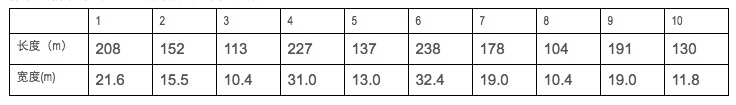
  Let's say we collect some longitude and latitude data for some warships.

  

  Based on this data, we used Python to draw a scatter plot:

  

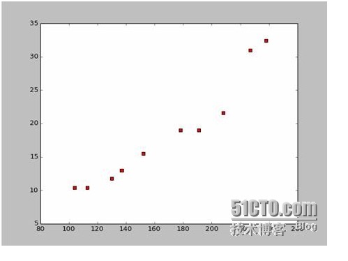
  The code for drawing the dotted line is as follows:

  import numpy as np                # -*- coding: utf-8 -*
  import os
  import matplotlib.pyplot as plt
  def drawScatterDiagram(fileName): # 改变工作路径到数据文件存放的地方
      os.chdir("d:/workspace_ml")
      xcord=[];ycord=[]
      fr=open(fileName)
      for line in fr.readlines():
          lineArr=line.strip().split()
          xcord.append(float(lineArr[1]));ycord.append(float(lineArr[2]))
      plt.scatter(xcord,ycord,s=30,c='red',marker='s')
      plt.show()
  

  So if we take the first two points of 238, 32.4, 152, 15.5, we get two equations. 152 peoplea+b=15.5 328A plus b is equal to 32.4. So let's solve these two equations for a is equal to 0.197, and b is equal to -14.48. So we can get a symmetry graph like this:

  

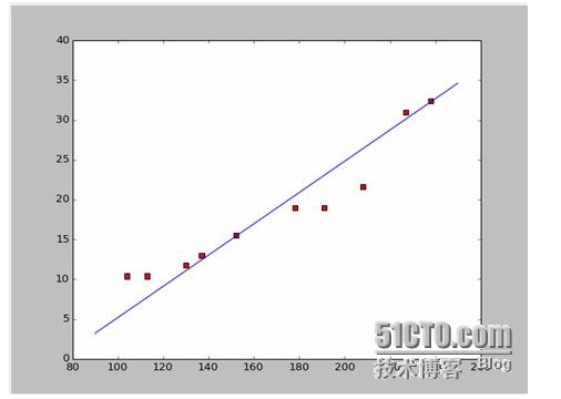
  OK, so here's a new question, is a and b optimal? The professional definition is: is a and b the optimal parameters of the model?

  The answer is: guarantee the square and the minimum of all the data deviations. As for the principle, we'll talk about it later, first we'll see how to use this tool to best calculate a and b. Assuming the square of all the data and is M,

  

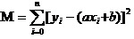
  Now what we're going to do is we're going to try to make M the smallest of a and b.

  So the equation is a binary function with (a, b) as the independent variable and (M) as the dependent variable.

  Recall that in higher numbers the value of the one-to-one function is extreme. We use the derivative tool. So in binary functions, we still use the derivative. But here the derivative has a new name. So if we take the derivative of M, we get a set of equations.

  

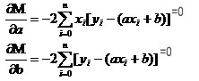
  In both equations, both x and y are known.

  It's easy to get a and b. Since I'm using Wikipedia data, I'm going to draw a picture directly from the answer:

  

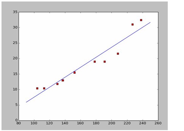
  # -*- coding: utf-8 -*importnumpy as npimportosimportmatplotlib.pyplot as pltdefdrawScatterDiagram(fileName):
  # 改变工作路径到数据文件存放的地方os.chdir("d:/workspace_ml")xcord=[];
  # ycord=[]fr=open(fileName)forline infr.readlines():lineArr=line.strip().split()xcord.append(float(lineArr[1]));
  # ycord.append(float(lineArr[2]))plt.scatter(xcord,ycord,s=30,c='red',marker='s')
  # a=0.1965;b=-14.486a=0.1612;b=-8.6394x=np.arange(90.0,250.0,0.1)y=a*x+bplt.plot(x,y)plt.show()
  # -*- coding: utf-8 -*
  import numpy as np
  import os
  import matplotlib.pyplot as plt
  def drawScatterDiagram(fileName):
      #改变工作路径到数据文件存放的地方
      os.chdir("d:/workspace_ml")
      xcord=[];ycord=[]
      fr=open(fileName)
      for line in fr.readlines():
          lineArr=line.strip().split()
          xcord.append(float(lineArr[1]));ycord.append(float(lineArr[2]))
      plt.scatter(xcord,ycord,s=30,c='red',marker='s')
      #a=0.1965;b=-14.486
      a=0.1612;b=-8.6394
      x=np.arange(90.0,250.0,0.1)
      y=a*x+b
      plt.plot(x,y)
      plt.show()
  

• Four, explore the basics

  In data matching, why optimize the model parameters by having the predicted data squared with the difference between the actual data rather than absolute and minimum values?

  This question has already been answered, see the link.http://blog.sciencenet.cn/blog-430956-621997.html）

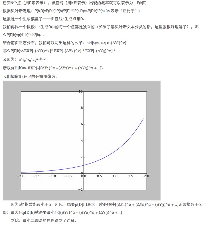
  I personally find this explanation very interesting. Especially the assumption that all points deviating from f (x) are noisy.

  The greater the deviation of a point, the smaller the probability that the point will occur. What is the relationship between the degree of deviation x and the probability of occurrence f (x)?

  

  

• Five, extend and extend

  All of the above are two-dimensional situations, i.e. there is only one independent variable. But in the real world, the final result is influenced by the superposition of multiple factors, i.e. there are multiple cases of independent variables.

  For a general N-sublinear function, it is OK to query with the inverse matrix in the tangent linear algebra; as no suitable example has been found for the time being, it is left here as a derivative.

  Of course, nature is more about polynomial conformation than simple linearity, which is a higher content.

• References

  • The Higher Mathematical Dictionary (sixth edition) (published by Higher Education)
  • He is the founder of the Beijing University Press.
  • This is the first time I've seen this video.The least common multiple of two.
  • Wikipedia: Minimum of two multiples
  • ScienceNet: What is it?The smallest power of two?

Original work, reproduction is allowed, when reproducing, be sure to indicate the original source of the article in the form of hyperlinks, author information and this statement; otherwise, legal liability will be pursued.http://sbp810050504.blog.51cto.com/2799422/1269572