Estrategia de trading cuantitativo multifactorial que combina el impulso con el juicio de tendencias


Fecha de creación: 2023-11-23 14:58:57 Última modificación: 2023-11-23 14:58:57
Copiar: 0 Número de Visitas: 644
1
Seguir
1617
Seguidores

Estrategia de trading cuantitativo multifactorial que combina el impulso con el juicio de tendencias

Descripción general

Esta estrategia es una estrategia de comercio cuantitativa de tipo de juicio multifactorial que combina indicadores de dinámica y indicadores de tendencia. La estrategia determina la tendencia general y la dirección de la dinámica del mercado mediante el cálculo de una combinación matemática de varios promedios y emite señales de comercio en función de las condiciones de desvalorización.

Principio de estrategia

  1. Cálculo de promedios de varios grupos y indicadores de movimiento
    • Calcula el promedio de Harmonics, el promedio a corto plazo, el promedio a medio plazo y el promedio a largo plazo
    • Calcular las diferencias entre las medias para reflejar la tendencia de los cambios en los precios
    • Cálculo de la derivada de grado uno de cada promedio para reflejar la dinámica de los cambios en los precios
    • Calcular el indicador de las cuerdas de la raíz para determinar la dirección de la tendencia
  2. Indicadores de negociación de juicio integrado
    • Las operaciones de ponderación se basan en varios factores, como el indicador de movimiento y el indicador de tendencia.
    • Valores cercanos a los mínimos para juzgar el estado actual del mercado
    • Se emitió una señal para hacer más operaciones de corto plazo.

Análisis de las ventajas

  1. La precisión de las señales se mejora con el uso de múltiples factores.
    • Tener en cuenta todos los factores: precios, tendencias y dinámicas
    • Diferentes factores pueden tener diferentes pesos
  2. Parámetros ajustables para diferentes mercados
    • Parámetros de promedio, límites entre las zonas de negociación
    • Adaptabilidad a diferentes ciclos y condiciones del mercado
  3. La estructura del código es clara y fácil de entender
    • Especificación de nombre, comentario completo
    • Fácil de reutilizar y optimizar

Análisis de riesgos

  1. Optimización de parámetros muy difícil
    • Se requiere una gran cantidad de datos históricos para encontrar los parámetros óptimos
  2. La frecuencia de las transacciones puede ser demasiado alta
    • La combinación de varios factores puede generar demasiadas transacciones
  3. Efectos y relevancia para el mercado
    • Las estrategias de evaluación de tendencias son susceptibles a comportamientos irracionales

Dirección de optimización

  1. Añadir la lógica de stop loss
    • Evite las pérdidas más grandes de las conductas irracionales
  2. Ajuste de los parámetros de optimización
    • Buscar la combinación óptima de parámetros para mejorar la estabilidad de la estrategia
  3. Añadir elementos de aprendizaje automático
    • El uso de aprendizaje profundo para evaluar el estado actual del mercado y ayudar a la toma de decisiones estratégicas

Resumir

La estrategia utiliza una combinación multifactorial de indicadores de dinámica y indicadores de tendencia para juzgar el estado del mercado y emitir señales de negociación según el umbral establecido. La estrategia tiene la ventaja de ser altamente configurable, adaptarse a diferentes entornos de mercado y ser fácil de entender. La desventaja es que la optimización de los parámetros es difícil, la frecuencia de negociación puede ser demasiado alta y el efecto es muy relevante para el mercado.
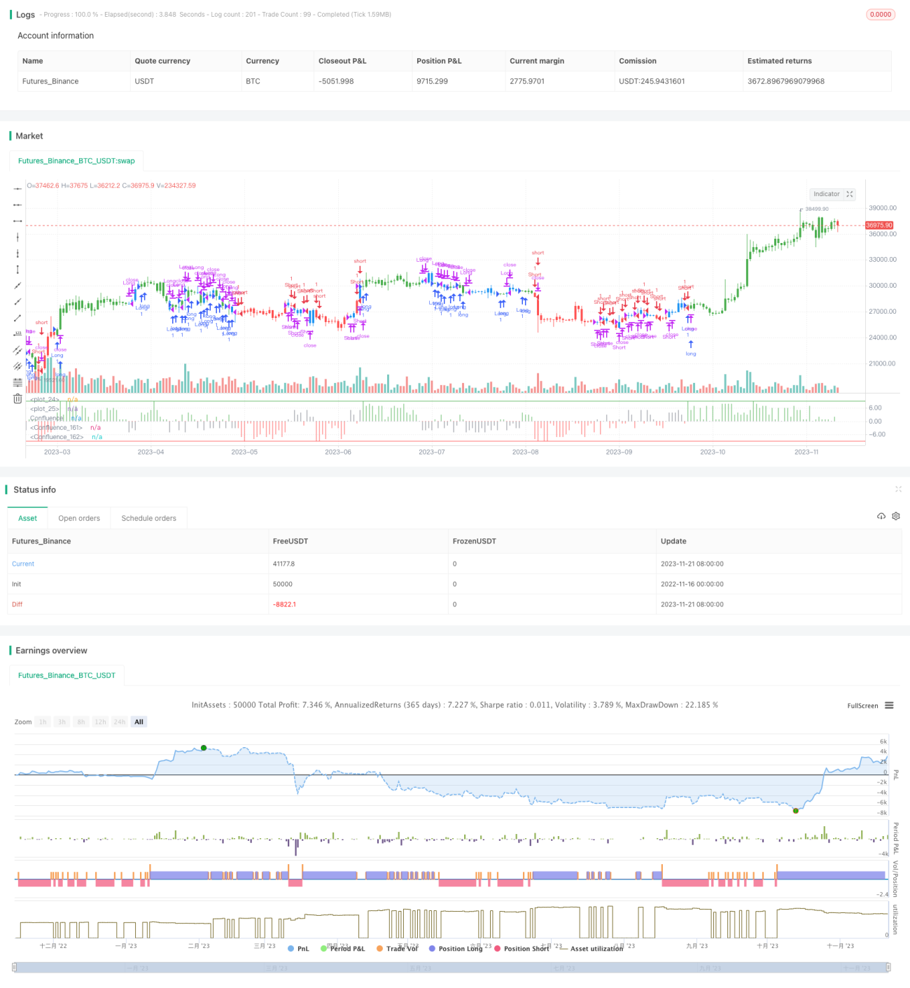
Código Fuente de la Estrategia
/*backtest
start: 2022-11-16 00:00:00
end: 2023-11-22 00:00:00
period: 1d
basePeriod: 1h
exchanges: [{"eid":"Futures_Binance","currency":"BTC_USDT"}]
*/

//@version=2
////////////////////////////////////////////////////////////
//  Copyright by HPotter v1.0 14/03/2017
// This is modified version of Dale Legan's "Confluence" indicator written by Gary Fritz.
// ================================================================
// Here is Gary`s commentary:
// Since the Confluence indicator returned several "states" (bull, bear, grey, and zero), 
// he modified the return value a bit:
// -9 to -1 = Bearish
// -0.9 to 0.9 = "grey" (and zero)
// 1 to 9 = Bullish
// The "grey" range corresponds to the "grey" values plotted by Dale's indicator, but 
// they're divided by 10.
//
// You can change long to short in the Input Settings
// Please, use it only for learning or paper trading. Do not for real trading.
////////////////////////////////////////////////////////////

strategy(title="Confluence", shorttitle="Confluence")
Harmonic = input(10, minval=1)
BuyBand = input(9)
SellBand = input(-9)
reverse = input(false, title="Trade reverse")
hline(SellBand, color=red, linestyle=line)
hline(BuyBand, color=green, linestyle=line)

Price = close

STL = round((Harmonic * 2) - 1 - 0.5)
ITL = round((STL * 2) - 1 - 0.5)
LTL = round((ITL * 2) - 1 - 0.5)
HOFF = round(Harmonic / 2 - 0.5)
SOFF = round(STL / 2 - 0.5)
IOFF = round(ITL / 2 - 0.5)

xHavg = sma(Price, Harmonic)
xSavg = sma(Price, STL)
xIavg = sma(Price, ITL)
xLavg = sma(Price, LTL)

xvalue2 = xSavg - xHavg[HOFF]
xvalue3 = xIavg - xSavg[SOFF]
xvalue12 = xLavg - xIavg[IOFF]

xmomsig = xvalue2 + xvalue3 + xvalue12

xLavgOHLC = sma(ohlc4, LTL - 1)

xH2 = sma(Price, Harmonic - 1)
xS2 = sma(Price, STL - 1)
xI2 = sma(Price, ITL - 1)
xL2 = sma(Price, LTL - 1)

DerivH = (xHavg * 2) - xHavg[1]
DerivS = (xSavg * 2) - xSavg[1]
DerivI = (xIavg * 2) - xIavg[1]
DerivL = (xLavg * 2) - xLavg[1]
SumDH = Harmonic * DerivH
SumDS = STL * DerivS
SumDI = ITL * DerivI
SumDL = LTL * DerivL

LengH = Harmonic - 1
LengS = STL - 1
LengI = ITL - 1
LengL = LTL - 1

N1H = xH2 * LengH
N1S = xS2 * LengS
N1I = xI2 * LengI
N1L = xL2 * LengL

DRH = SumDH - N1H
DRS = SumDS - N1S
DRI = SumDI - N1I
DRL = SumDL - N1L

SumH = xH2 * (Harmonic - 1)
SumS = xS2 * (STL - 1)
SumI = xI2 * (ITL - 1)
SumL = xLavgOHLC * (LTL - 1)

xvalue5 = (SumH + DRH) / Harmonic
xvalue6 = (SumS + DRS) / STL
xvalue7 = (SumI + DRI) / ITL
xvalue13 = (SumL + DRL) / LTL

value9 = xvalue6 - xvalue5[HOFF]
value10 = xvalue7 - xvalue6[SOFF]
value14 = xvalue13 - xvalue7[IOFF]
xmom = value9 + value10 + value14

HT = sin(xvalue5 * 2 * 3.14 / 360) + cos(xvalue5 * 2 * 3.14 / 360)
HTA = sin(xHavg * 2 * 3.14 / 360) + cos(xHavg * 2 * 3.14 / 360)
ST = sin(xvalue6 * 2 * 3.14 / 360) + cos(xvalue6 * 2 * 3.14 / 360)
STA = sin(xSavg * 2 * 3.14 / 360) + cos(xSavg * 2 * 3.14 / 360)
IT = sin(xvalue7 * 2 * 3.14 / 360) + cos(xvalue7 * 2 * 3.14 / 360)
ITA = sin(xIavg * 2 * 3.14 / 360) + cos(xIavg * 2 * 3.14 / 360)

xSum = HT + ST + IT
xErr = HTA + STA + ITA

Condition2 = (((xSum > xSum[SOFF]) and (xHavg < xHavg[SOFF])) or ((xSum < xSum[SOFF]) and (xHavg > xHavg[SOFF])))
Phase = iff(Condition2 , -1 , 1)
xErrSum = (xSum - xErr) * Phase
xErrSig = sma(xErrSum, SOFF)

xvalue70 = xvalue5 - xvalue13
xvalue71 = sma(xvalue70, Harmonic)


ErrNum = iff (xErrSum > 0 and xErrSum < xErrSum[1] and xErrSum < xErrSig, 1,
          iff (xErrSum > 0 and xErrSum < xErrSum[1] and xErrSum > xErrSig, 2, 
           iff (xErrSum > 0 and xErrSum > xErrSum[1] and xErrSum < xErrSig, 2,
             iff (xErrSum > 0 and xErrSum > xErrSum[1] and xErrSum > xErrSig, 3,
              iff (xErrSum < 0 and xErrSum > xErrSum[1] and xErrSum > xErrSig, -1,
               iff (xErrSum < 0 and xErrSum < xErrSum[1] and xErrSum > xErrSig, -2,
                 iff (xErrSum < 0 and xErrSum > xErrSum[1] and xErrSum < xErrSig, -2,
                  iff (xErrSum < 0 and xErrSum < xErrSum[1] and xErrSum < xErrSig, -3, 0))))))))


momNum = iff (xmom > 0 and xmom < xmom[1] and xmom < xmomsig , 1,
          iff (xmom > 0 and xmom < xmom[1] and xmom > xmomsig, 2,
           iff (xmom > 0 and xmom > xmom[1] and xmom < xmomsig, 2,
             iff (xmom > 0 and xmom > xmom[1] and xmom > xmomsig, 3,
              iff (xmom < 0 and xmom > xmom[1] and xmom > xmomsig, -1,
               iff (xmom < 0 and xmom < xmom[1] and xmom > xmomsig, -2,
                 iff (xmom < 0 and xmom > xmom[1] and xmom < xmomsig, -2,
                  iff (xmom < 0 and xmom < xmom[1] and xmom < xmomsig, -3, 0))))))))

TCNum =  iff (xvalue70 > 0 and xvalue70 < xvalue70[1] and xvalue70 < xvalue71, 1,
          iff (xvalue70 > 0 and xvalue70 < xvalue70[1] and xvalue70 > xvalue71, 2,
           iff (xvalue70 > 0 and xvalue70 > xvalue70[1] and xvalue70 < xvalue71, 2,
             iff (xvalue70 > 0 and xvalue70 > xvalue70[1] and xvalue70 > xvalue71, 3,
              iff (xvalue70 < 0 and xvalue70 > xvalue70[1] and xvalue70 > xvalue71, -1,
               iff (xvalue70 < 0 and xvalue70 < xvalue70[1] and xvalue70 > xvalue71, -2,
                 iff (xvalue70 < 0 and xvalue70 > xvalue70[1] and xvalue70 < xvalue71, -2,
                  iff (xvalue70 < 0 and xvalue70 < xvalue70[1] and xvalue70 < xvalue71, -3,0))))))))

value42 = ErrNum + momNum + TCNum
Confluence = iff (value42 > 0 and xvalue70 > 0, value42,
              iff (value42 < 0 and xvalue70 < 0, value42,
               iff ((value42 > 0 and xvalue70 < 0) or (value42 < 0 and xvalue70 > 0), value42 / 10, 0)))
Res1 = iff (Confluence >= 1, Confluence, 0)
Res2 = iff (Confluence <= -1, Confluence, 0)
Res3 = iff (Confluence == 0, 0, iff (Confluence > -1 and Confluence < 1, 10 * Confluence, 0))
pos = iff(Res2 >= SellBand and Res2 != 0, -1,
	     iff(Res1 <= BuyBand and Res1 != 0, 1, 
	       iff(Res3 != 0, 0, nz(pos[1], 0))))
possig = iff(reverse and pos == 1, -1,
          iff(reverse and pos == -1, 1, pos))	   
if (possig == 1) 
    strategy.entry("Long", strategy.long)
if (possig == -1)
    strategy.entry("Short", strategy.short)	   	 
if (possig == 0)
    strategy.close("Long", when = possig == 0)	 
    strategy.close("Short", when = possig == 0)	 
barcolor(possig == -1 ? red: possig == 1 ? green : blue )
plot(Res1, color=green, title="Confluence", linewidth=3, style = histogram)
plot(Res2, color=red, title="Confluence", linewidth=3, style = histogram)
plot(Res3, color=gray, title="Confluence",  linewidth=3, style = histogram)