Estrategia de negociación de Bitcoin basada en indicadores cuantitativos

El autor:¿ Qué pasa?, Fecha: 2023-12-26 11:06:12
Las etiquetas:

Resumen general

Esta estrategia utiliza múltiples indicadores cuantitativos para determinar el momento de compra y venta de Bitcoin y automatizar la negociación.

Principio de la estrategia

Utilice el promedio móvil de Hull modificado para determinar la dirección de tendencia principal del mercado, combinado con bandas de Bollinger para ayudar a determinar los puntos de compra y venta de ruptura.
El indicador RSI combinado con un rango de volatilidad adaptativo determina las zonas de sobrecompra y sobreventa para generar señales comerciales.
El oscilador de volumen determina el impulso de compra y venta para evitar falsos breakouts.
Establecer las relaciones stop loss/take profit con antelación para establecer previamente los niveles de stop loss y take profit para la gestión del riesgo.

Análisis de ventajas

La curva de Hull puede capturar los cambios de tendencia más rápidamente, y las bandas de Bollinger pueden ayudar a reducir las señales falsas.
La optimización de los parámetros del RSI y la verificación de señales duplicadas lo hacen más confiable.
El oscilador de volumen combinado con las tendencias y las señales de indicadores evita operaciones inexactas.
Los métodos de stop loss y take profit preestablecidos pueden controlar automáticamente las ganancias y pérdidas individuales y gestionar eficazmente el riesgo general.

Análisis de riesgos

La configuración incorrecta de los parámetros puede dar lugar a una frecuencia de negociación demasiado alta o a un deterioro del rendimiento de la señal.
Los acontecimientos repentinos del mercado pueden hacer que los precios fluctúen violentamente, lo que resulta en el inicio de un stop loss y mayores pérdidas.
Cuando la variedad de comercio se cambia a otras monedas, los parámetros deben volver a probarse y optimizarse.
Si faltan datos de volumen, el oscilador de volumen fallará.

Direcciones de optimización

Prueba más combinaciones de parámetros RSI para encontrar los parámetros óptimos.
Intenta combinar el RSI con otros indicadores como el MACD y el KD para mejorar la precisión de la señal.
Añadir módulos de predicción de modelos y utilizar el aprendizaje automático para juzgar la dirección del mercado.
Prueba los parámetros cuando se aplican a otras variedades comerciales.
Optimice los algoritmos de stop loss y take profit para maximizar los beneficios.

Resumen de las actividades

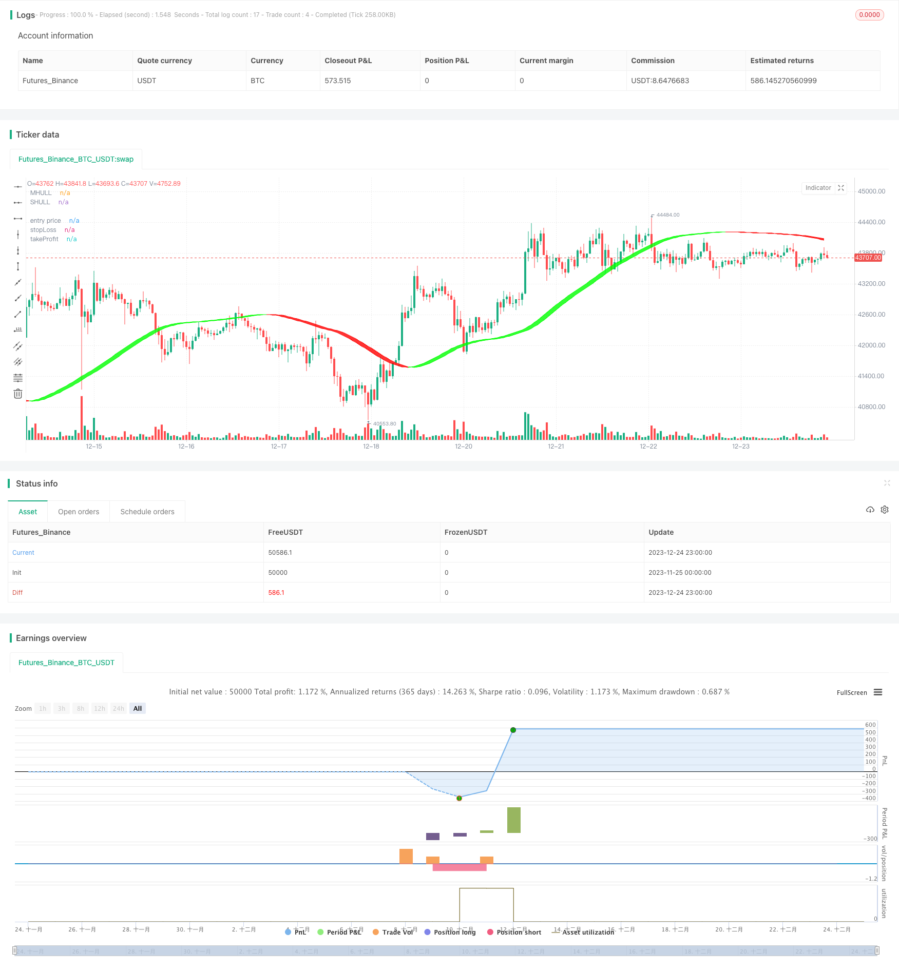
Esta estrategia combina múltiples indicadores técnicos cuantitativos para determinar el momento de entrada y salida. A través de la optimización de parámetros, el control de riesgos y otros métodos, ha logrado el comercio automatizado de Bitcoin con buenos resultados. Pero aún requiere pruebas y optimización continuas para adaptarse a los cambios del mercado. Puede servir como referencia para que los inversores ayuden en las decisiones comerciales.

/*backtest
start: 2023-11-25 00:00:00
end: 2023-12-25 00:00:00
period: 1h
basePeriod: 15m
exchanges: [{"eid":"Futures_Binance","currency":"BTC_USDT"}]
*/


// © maxencetajet

//@version=5
strategy("Strategy Crypto", overlay=true, initial_capital=1000, default_qty_type=strategy.fixed, default_qty_value=0.5, slippage=25)

src1 = input.source(close, title="Source")
target_stop_ratio = input.float(title='Risk/Reward', defval=1.5, minval=0.5, maxval=100)

startDate = input.int(title='Start Date', defval=1, minval=1, maxval=31, group="beginning Backtest")
startMonth = input.int(title='Start Month', defval=5, minval=1, maxval=12, group="beginning Backtest")
startYear = input.int(title='Start Year', defval=2022, minval=2000, maxval=2100, group="beginning Backtest")

inDateRange = time >= timestamp(syminfo.timezone, startYear, startMonth, startDate, 0, 0)

swingHighV = input.int(7, title="Swing High", group="number of past candles")
swingLowV = input.int(7, title="Swing Low", group="number of past candles")

//Hull Suite

modeSwitch = input.string("Hma", title="Hull Variation", options=["Hma", "Thma", "Ehma"], group="Hull Suite")
length = input(60, title="Length", group="Hull Suite")
lengthMult = input(3, title="Length multiplier", group="Hull Suite")

HMA(_src1, _length) =>
    ta.wma(2 * ta.wma(_src1, _length / 2) - ta.wma(_src1, _length), math.round(math.sqrt(_length)))

EHMA(_src1, _length) =>
    ta.ema(2 * ta.ema(_src1, _length / 2) - ta.ema(_src1, _length), math.round(math.sqrt(_length)))

THMA(_src1, _length) =>
    ta.wma(ta.wma(_src1, _length / 3) * 3 - ta.wma(_src1, _length / 2) - ta.wma(_src1, _length), _length)

Mode(modeSwitch, src1, len) =>
    modeSwitch == 'Hma' ? HMA(src1, len) : modeSwitch == 'Ehma' ? EHMA(src1, len) : modeSwitch == 'Thma' ? THMA(src1, len / 2) : na

_hull = Mode(modeSwitch, src1, int(length * lengthMult))
HULL = _hull
MHULL = HULL[0]
SHULL = HULL[2]

hullColor = HULL > HULL[2] ? #00ff00 : #ff0000

Fi1 = plot(MHULL, title='MHULL', color=hullColor, linewidth=1, transp=50)
Fi2 = plot(SHULL, title='SHULL', color=hullColor, linewidth=1, transp=50)
fill(Fi1, Fi2, title='Band Filler', color=hullColor, transp=40)

//QQE MOD

RSI_Period = input(6, title='RSI Length', group="QQE MOD")
SF = input(5, title='RSI Smoothing', group="QQE MOD")
QQE = input(3, title='Fast QQE Factor', group="QQE MOD")
ThreshHold = input(3, title='Thresh-hold', group="QQE MOD")

src = input(close, title='RSI Source', group="QQE MOD")

Wilders_Period = RSI_Period * 2 - 1

Rsi = ta.rsi(src, RSI_Period)
RsiMa = ta.ema(Rsi, SF)
AtrRsi = math.abs(RsiMa[1] - RsiMa)
MaAtrRsi = ta.ema(AtrRsi, Wilders_Period)
dar = ta.ema(MaAtrRsi, Wilders_Period) * QQE

longband = 0.0
shortband = 0.0
trend = 0

DeltaFastAtrRsi = dar
RSIndex = RsiMa
newshortband = RSIndex + DeltaFastAtrRsi
newlongband = RSIndex - DeltaFastAtrRsi
longband := RSIndex[1] > longband[1] and RSIndex > longband[1] ? math.max(longband[1], newlongband) : newlongband
shortband := RSIndex[1] < shortband[1] and RSIndex < shortband[1] ? math.min(shortband[1], newshortband) : newshortband
cross_1 = ta.cross(longband[1], RSIndex)
trend := ta.cross(RSIndex, shortband[1]) ? 1 : cross_1 ? -1 : nz(trend[1], 1)
FastAtrRsiTL = trend == 1 ? longband : shortband

length1 = input.int(50, minval=1, title='Bollinger Length', group="QQE MOD")
mult = input.float(0.35, minval=0.001, maxval=5, step=0.1, title='BB Multiplier', group="QQE MOD")
basis = ta.sma(FastAtrRsiTL - 50, length1)
dev = mult * ta.stdev(FastAtrRsiTL - 50, length1)
upper = basis + dev
lower = basis - dev
color_bar = RsiMa - 50 > upper ? #00c3ff : RsiMa - 50 < lower ? #ff0062 : color.gray

QQEzlong = 0
QQEzlong := nz(QQEzlong[1])
QQEzshort = 0
QQEzshort := nz(QQEzshort[1])
QQEzlong := RSIndex >= 50 ? QQEzlong + 1 : 0
QQEzshort := RSIndex < 50 ? QQEzshort + 1 : 0

RSI_Period2 = input(6, title='RSI Length', group="QQE MOD")
SF2 = input(5, title='RSI Smoothing', group="QQE MOD")
QQE2 = input(1.61, title='Fast QQE2 Factor', group="QQE MOD")
ThreshHold2 = input(3, title='Thresh-hold', group="QQE MOD")

src2 = input(close, title='RSI Source', group="QQE MOD")

Wilders_Period2 = RSI_Period2 * 2 - 1

Rsi2 = ta.rsi(src2, RSI_Period2)
RsiMa2 = ta.ema(Rsi2, SF2)
AtrRsi2 = math.abs(RsiMa2[1] - RsiMa2)
MaAtrRsi2 = ta.ema(AtrRsi2, Wilders_Period2)
dar2 = ta.ema(MaAtrRsi2, Wilders_Period2) * QQE2
longband2 = 0.0
shortband2 = 0.0
trend2 = 0

DeltaFastAtrRsi2 = dar2
RSIndex2 = RsiMa2
newshortband2 = RSIndex2 + DeltaFastAtrRsi2
newlongband2 = RSIndex2 - DeltaFastAtrRsi2
longband2 := RSIndex2[1] > longband2[1] and RSIndex2 > longband2[1] ? math.max(longband2[1], newlongband2) : newlongband2
shortband2 := RSIndex2[1] < shortband2[1] and RSIndex2 < shortband2[1] ? math.min(shortband2[1], newshortband2) : newshortband2
cross_2 = ta.cross(longband2[1], RSIndex2)
trend2 := ta.cross(RSIndex2, shortband2[1]) ? 1 : cross_2 ? -1 : nz(trend2[1], 1)
FastAtrRsi2TL = trend2 == 1 ? longband2 : shortband2

QQE2zlong = 0
QQE2zlong := nz(QQE2zlong[1])
QQE2zshort = 0
QQE2zshort := nz(QQE2zshort[1])
QQE2zlong := RSIndex2 >= 50 ? QQE2zlong + 1 : 0
QQE2zshort := RSIndex2 < 50 ? QQE2zshort + 1 : 0

hcolor2 = RsiMa2 - 50 > ThreshHold2 ? color.silver : RsiMa2 - 50 < 0 - ThreshHold2 ? color.silver : na

Greenbar1 = RsiMa2 - 50 > ThreshHold2
Greenbar2 = RsiMa - 50 > upper

Redbar1 = RsiMa2 - 50 < 0 - ThreshHold2
Redbar2 = RsiMa - 50 < lower

//Volume Oscillator

var cumVol = 0.
cumVol += nz(volume)
if barstate.islast and cumVol == 0
    runtime.error("No volume is provided by the data vendor.")
shortlen = input.int(5, minval=1, title = "Short Length", group="Volume Oscillator")
longlen = input.int(10, minval=1, title = "Long Length", group="Volume Oscillator")
short = ta.ema(volume, shortlen)
long = ta.ema(volume, longlen)
osc = 100 * (short - long) / long

//strategy

enterLong   =  '    {  "message_type": "bot",  "bot_id": 4635591,  "email_token": "25byourtefcodeuufyd2-43314-ab98-bjorg224",  "delay_seconds": 1}  ' //start long deal
 
ExitLong    =  '    {  "message_type": "bot",  "bot_id": 4635591,  "email_token": "25byourtefcodeuufyd2-43314-ab98-bjorg224",  "delay_seconds": 0,  "action": "close_at_market_price"}  ' // close long deal market 
 
enterShort  =  '    {  "message_type": "bot",  "bot_id": 4635690,  "email_token": "25byourtefcodeuufyd2-43314-ab98-bjorg224",  "delay_seconds": 1}  ' // start short deal
 
ExitShort   =  '    {  "message_type": "bot",  "bot_id": 4635690,  "email_token": "25byourtefcodeuufyd2-43314-ab98-bjorg224",  "delay_seconds": 0,  "action": "close_at_market_price"}  ' // close short deal market

longcondition = close > MHULL and HULL > HULL[2] and osc > 0 and Greenbar1 and Greenbar2 and not Greenbar1[1] and not Greenbar2[1]
shortcondition = close < SHULL and HULL < HULL[2] and osc > 0 and Redbar1 and Redbar2 and not Redbar1[1] and not Redbar2[1]

float risk_long = na
float risk_short = na
float stopLoss = na
float takeProfit = na
float entry_price = na

risk_long := risk_long[1]
risk_short := risk_short[1]

swingHigh = ta.highest(high, swingHighV)
swingLow = ta.lowest(low, swingLowV)

if strategy.position_size == 0 and longcondition and inDateRange
    risk_long := (close - swingLow) / close
    strategy.entry("long", strategy.long, comment="Buy", alert_message=enterLong)
    
if strategy.position_size == 0 and shortcondition and inDateRange
    risk_short := (swingHigh - close) / close       
    strategy.entry("short", strategy.short, comment="Sell", alert_message=enterShort)
    
if strategy.position_size > 0

    stopLoss := strategy.position_avg_price * (1 - risk_long)
    takeProfit := strategy.position_avg_price * (1 + target_stop_ratio * risk_long)
    entry_price := strategy.position_avg_price
    strategy.exit("long exit", "long", stop = stopLoss, limit = takeProfit, alert_message=ExitLong)
    
if strategy.position_size < 0

    stopLoss := strategy.position_avg_price * (1 + risk_short)
    takeProfit := strategy.position_avg_price * (1 - target_stop_ratio * risk_short)
    entry_price := strategy.position_avg_price
    strategy.exit("short exit", "short", stop = stopLoss, limit = takeProfit, alert_message=ExitShort)

p_ep = plot(entry_price, color=color.new(color.white, 0), linewidth=2, style=plot.style_linebr, title='entry price')
p_sl = plot(stopLoss, color=color.new(color.red, 0), linewidth=2, style=plot.style_linebr, title='stopLoss')
p_tp = plot(takeProfit, color=color.new(color.green, 0), linewidth=2, style=plot.style_linebr, title='takeProfit')
fill(p_sl, p_ep, color.new(color.red, transp=85))
fill(p_tp, p_ep, color.new(color.green, transp=85))

Más.