[TOC]

Posted in: Community > Crypto Market RWA Multi-Asset Dynamic Weight Allocation: Risk Parity Strategy

The crypto market hasn’t been easy lately. BTC has pulled back hard from the highs, altcoins have been hit even worse, and a lot of people are sitting on the sidelines or leaving altogether. But during this same stretch, something else has been quietly heating up — RWA, the tokenization of real-world assets. Gold, US equities, crude oil — assets from traditional markets are starting to show up on crypto exchanges in contract form. Major exchanges have rolled out SPY (tracking the S&P 500 ETF), gold XAU, crude CL, and so on. Combined with BTC, which was already there, a multi-asset trading environment covering US equities, gold, crude oil, and crypto has taken shape on-chain for the first time.

Looking at this lineup, an idea came to mind: traditional finance has a classic approach called risk parity. In plain terms — don’t put all your eggs in one basket, and how much you put in each basket depends on how risky that basket is. This logic has been used in traditional finance circles for decades. In a bear market like this one, everyone is looking for ways to not depend on a single asset for survival. Now that the crypto market finally has contracts for these assets, it’s time to port that logic over and give it a try.

Getting Risk Parity Straight First

Before getting into the specifics, it’s worth explaining what “risk parity” actually means, otherwise the logic that follows is hard to track.

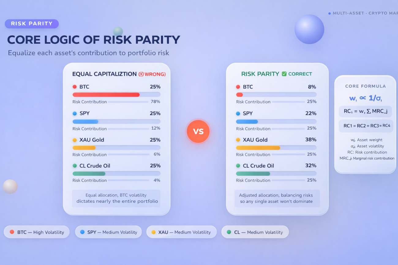
A normal person allocating assets might think: I’ll split my money evenly into four parts, 25% per asset. Sounds balanced, but the problem is that BTC can swing 10% in a day while gold might move 0.5%. With the same 25% allocation, BTC brings you twenty times the risk that gold does. On the surface the four assets are split evenly, but in reality the portfolio’s fate is almost entirely determined by BTC alone — the other three are just there for show.

Risk parity flips this around: don’t split the money evenly, split the risk evenly. BTC is volatile, so allocate less to it; gold is stable, so allocate more — but that’s only step one. The more critical piece is that assets aren’t independent of one another. BTC and US equities can fall together under certain conditions. If two assets move strongly in the same direction, spreading risk between them is of limited value even if their individual volatilities differ. True risk parity has to simultaneously account for each asset’s volatility and its correlation with the others, using the covariance matrix to measure each asset’s marginal contribution to total portfolio risk, so that each asset ends up contributing roughly the same amount of risk. The upside of this logic is that a sudden blowup in any single asset won’t take down the whole portfolio.

Pick the Right Assets First — Diversification Only Makes Sense If You Do

To do risk parity, the first thing is picking what goes in the basket. If the asset selection is wrong, no amount of calculation precision downstream will help.

The asset pool chosen was SPY, XAU, CL, and BTC. There’s a logic to picking these four — they don’t usually move in lockstep. Equities rise when the economy is good, gold rallies when risk-off sentiment picks up, crude and gold both move on inflation expectations, and crypto sometimes tracks equities and sometimes goes completely off-script. It’s precisely because their correlations are low that putting them together actually diversifies risk. If all four went up and down together every day, “diversification” would be an illusion, and no method could save you.

Once the assets are chosen, the next question is: how much to put in each? That’s what risk parity actually needs to calculate.

How to Compute Each Asset’s Weight

The strategy’s computation is a two-step process.

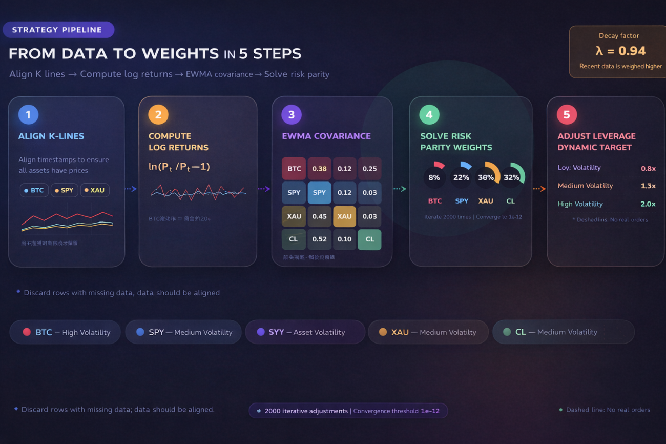
Step one: pull K-line data for the four assets and align by timestamp. The strategy uses 1-hour K-lines (PERIOD_H1) as its data input. This step looks simple, but in reality RWA contract products sometimes have missing data. If SPY has no quote at some timestamp, that entire row is dropped — only timestamps where all four assets have quotes are kept for later calculations.

for (var k = 0; k < keys.length; k++) {
    var row = timeMap[keys[k]], ok = true;
    for (var i = 0; i < LABELS.length; i++) {
        if (row[LABELS[i]] === undefined) { ok = false; break; }
    }
    if (ok) timestamps.push(parseInt(keys[k]));
}

After alignment, closing price series are converted into log returns — that is, ln(current price / previous price). Log returns are used instead of simple percentage changes because they have time additivity — returns across multiple periods can be summed directly to get the total log return, which is easier to handle. Also, under the common assumption that asset prices follow geometric Brownian motion, log returns are normally distributed, which is compatible with the covariance matrix framework that follows. One caveat worth noting: actual returns on crypto assets tend to have fat tails, which is a known assumption bias — the covariance matrix can underestimate real risk in extreme conditions.

function calcLogReturns(prices) {
    var r = [];
    for (var i = 1; i < prices.length; i++) {
        var prev = prices[i - 1], cur = prices[i];
        if (!prev || !cur || prev <= 0 || cur <= 0) { r.push(0); continue; }
        r.push(Math.log(cur / prev));
    }
    return r;
}

Step two: use these return series to compute the covariance matrix. Just using the plain historical average covariance is too crude — what’s used here is EWMA (exponentially weighted) — giving recent data higher weights so the covariance matrix can pick up on changes in market regime more quickly.

for (var t = T - 1; t >= 0; t--) {
    var w = Math.pow(lambda, T - 1 - t);
    c += w * (retMat[i][t] - means[i]) * (retMat[j][t] - means[j]);
    ws += w;
}
cov[i][j] = c / ws;
cov[j][i] = cov[i][j];

lambda is the decay coefficient, and the strategy uses EWMA_LAMBDA = 0.94 by default — a value drawn from RiskMetrics’ empirical setting for daily data. Note that RiskMetrics’ 0.94 was designed for daily data, while the strategy uses 1-hour data at a higher frequency. If you want the covariance matrix’s sensitivity to recent changes to match that of daily 0.94, in theory it should be converted to a value closer to 1. But in practice, 0.94 is still a reasonable starting point at the hourly level — it represents a configuration where recent data gets higher weights and historical data decays faster. You can adjust it based on actual backtest results. The closer lambda is to 1, the more persistent the historical data’s influence becomes, and the slower the covariance matrix reacts to recent changes. The smaller lambda is, the more responsive the strategy is to regime changes, but it also becomes more prone to triggering unnecessary rebalances due to short-term noise.

After the calculation, a regularization term is added to the diagonal, with a coefficient of 0.1% of the diagonal mean (eps = diagMean * 0.001). The 0.001 multiplier was chosen through testing — numerically sufficient to ensure positive definiteness of the matrix, while its impact on the covariance structure is negligible. One simplification worth noting: the strict form of EWMA covariance should use a weighted mean for computing deviations, but the code uses the simple arithmetic mean over the entire lookback window. When return means are close to zero (the common state of short-term financial asset returns), this simplification has negligible impact on results, but it introduces a small bias when means deviate significantly from zero.

With the covariance matrix in hand, the next step is the actual risk parity solver — finding a set of weights where each asset contributes roughly equally to portfolio risk. Before iteration begins, the strategy has already determined the direction of each asset through the covariance of an equal-volatility portfolio, with results stored in the signs[] array (+1 for long, -1 for short). The iteration process uses these pre-determined fixed signs throughout, adjusting only the magnitude of the weights without changing direction — this is done for engineering stability, to prevent weights from repeatedly flipping direction during iteration due to numerical perturbation.

There’s no analytical solution to this problem, so it’s approached iteratively. Each round computes the current risk contributions, pushes down the weights of assets contributing too much, lifts up the weights of those contributing too little, and repeats until convergence.

for (var iter = 0; iter < 2000; iter++) {
    var trc = riskContribs(w, scaledCov);
    var pv = portVol(w, scaledCov);
    var target = pv / n;
    var obj = 0;
    for (var i = 0; i < n; i++) {
        for (var j = i + 1; j < n; j++) {
            var d = Math.abs(trc[i]) - Math.abs(trc[j]);
            obj += d * d;
        }
    }
    if (obj < 1e-12) break;
    var nw = [], ns = 0;
    for (var i = 0; i < n; i++) {
        var rc = Math.abs(trc[i]);
        var sign = signs[i]; // use the pre-determined fixed sign
        var a = target / rc;
        var v = sign * Math.max(Math.abs(w[i]) * Math.pow(a, 0.5), 1e-6);
        nw.push(v);
        ns += Math.abs(v);
    }
    // Absolute-value normalization: the sum of absolute weights equals 1
    for (var i = 0; i < n; i++) w[i] = nw[i] / ns;
}

The convergence criterion is that the sum of squared differences in risk contributions across all assets is below 1e-12, at which point risk contributions are considered close enough and iteration stops. The maximum iteration count is capped at 2000 to prevent infinite loops when the covariance matrix is ill-conditioned. In practice convergence usually happens within a few hundred iterations. If it hasn’t converged by the cap, it means there’s something wrong with the input data or the covariance matrix — in that case the strategy falls back to an equal-weight long portfolio, ensuring the system doesn’t idle.

Each asset’s risk contribution is defined as its weight multiplied by its marginal risk — the result can be negative, meaning the asset is reducing overall portfolio volatility.

function riskContribs(w, cov) {
    var sv = matVecMul(cov, w);
    var pv = portVol(w, cov);
    var trc = [];
    for (var i = 0; i < w.length; i++) trc.push(w[i] * sv[i] / pv);
    return trc;
}

Weights Can Be Negative — i.e. Shorting Is Allowed

Standard risk parity strategies are typically long-only, but the contract market allows shorting, so the strategy extends this by letting weights be negative.

The logic is this: first compute an equal-volatility reference portfolio — high-volatility assets get low weights, low-volatility assets get high weights — then check whether each asset’s covariance with this reference portfolio is positive or negative. If the covariance is negative, it means this asset tends to move inversely to the portfolio overall, so shorting it helps reduce total portfolio risk. The weight is set negative, which corresponds to opening a short position in the contract market.

One caveat: this is an engineering approximation, not the canonical solution from long-short risk parity theory. Strict long-short risk parity requires constrained optimization based on the full covariance matrix, at higher computational cost. The approximation here gives reasonable directional judgments under most market conditions, but when multiple assets simultaneously have negative covariance with the reference portfolio, whether shorting all of them at once still reduces total portfolio risk needs to be verified case by case and cannot be taken for granted.

var invVols = [], sumInvVol = 0;
for (var i = 0; i < n; i++) {
    var vol = Math.sqrt(Math.max(scaledCov[i][i], 1e-16));
    invVols.push(1 / vol);
    sumInvVol += 1 / vol;
}
var eqVolWeights = [];
for (var i = 0; i < n; i++) {
    eqVolWeights.push(invVols[i] / sumInvVol);
}
var covWithPortfolio = 0;
for (var j = 0; j < n; j++) {
    covWithPortfolio += eqVolWeights[j] * scaledCov[i][j];
}
var dir = covWithPortfolio < 0 ? -1 : 1;
Log('[Direction]', LABELS[i], 'covariance with equal-vol portfolio:',
    _N(covWithPortfolio, 8), '→', dir < 0 ? '🔴 short' : '🟢 long');

Once the direction is determined, it’s stored in the signs[] array and never changes during the entire iterative solving process. The iteration only adjusts the magnitudes of the weights — direction stays fixed. With direction settled, there’s still one more thing to handle: how much leverage the overall portfolio should carry.

Leverage Isn’t About Going Higher — It Follows Volatility

The strategy has a built-in leverage adjustment mechanism aimed at keeping portfolio volatility near a preset target. An analogy: you’re driving, target speed 60 km/h. On a clear highway you can press the gas a little harder; in heavy city traffic you ease off. The strategy’s leverage mechanism works similarly — when overall market volatility is low, leverage is dialed up to bring portfolio risk to target; when volatility is high, leverage is automatically reduced and exposure contracts.

The strategy uses 1-hour K-lines, and there are exactly 8760 of them in a year, so the annualization factor is simply sqrt(8760). Switching to a different period means adjusting this factor: sqrt(35040) for 15-minute, sqrt(2190) for 4-hour, sqrt(365) for daily.

function calcLeverage(w, cov) {
    var pv = portVol(w, cov) * Math.sqrt(8760);
    if (!isFinite(pv) || pv <= 0) return 1;
    return Math.min(TARGET_VOL / pv, MAX_LEVERAGE);
}

Dividing portfolio annualized volatility by target volatility gives the leverage multiplier to apply, with a cap to prevent runaway leverage under extreme conditions. This isn’t about chasing maximum returns — it’s risk budgeting. How much risk is traded for how much return is decided in advance, not drifting with the market.

Once leverage is computed, the portfolio can open positions. At the same time, the strategy automatically adjusts the main loop’s polling interval based on current volatility — the higher the volatility, the faster the refresh; the lower the volatility, the slower the pace, reducing unnecessary computation and trading friction.

function getAdaptiveSleep(w, cov) {
    var av = portVol(w, cov) * Math.sqrt(8760);
    if (av > 0.50) return FAST_INTERVAL;   // 15 min
    else if (av > 0.30) return MID_INTERVAL; // 30 min
    else return SLOW_INTERVAL;               // 60 min
}

When to Rebalance

The market moves every day, and weights will continuously drift away from the original design. Left alone, over time the actual portfolio risk can diverge significantly from the intended level. The strategy sets two rebalance triggers: one is time-based — every fixed number of hours, weights are forcibly recomputed. The other is drift-based — when an asset’s actual weight deviates from its target weight beyond a threshold, or when its long/short direction flips, a rebalance is triggered immediately without waiting for the next scheduled one.

When computing relative drift, the denominator is the absolute value of the previous weight. If an asset’s weight has been squeezed very small (close to zero), relative drift is amplified and can trigger frequent rebalancing. The strategy has protection for this: when lastWeights[i] is zero, drift check is skipped to avoid false triggers from division by zero.

if (!lastWeights) {
    needRebal = true;
    rebalReason = 'Initial position build';
} else if ((now - lastTime) > REBALANCE_HOURS * 3600000) {
    needRebal = true;
    rebalReason = 'Scheduled rebalance (' + REBALANCE_HOURS + 'h)';
} else {
    for (var i = 0; i < weights.length; i++) {
        if ((weights[i] >= 0) !== (lastWeights[i] >= 0)) {
            needRebal = true;
            rebalReason = LABELS[i] + ' direction flip (long↔short)';
            break;
        }
        if (lastWeights[i] !== 0 &&
            Math.abs(weights[i] - lastWeights[i]) / Math.abs(lastWeights[i]) > DRIFT_THRESHOLD) {
            needRebal = true;
            rebalReason = LABELS[i] + ' weight drift exceeds threshold';
            break;
        }
    }
}

Once a rebalance is triggered, the strategy computes the target notional amount for each asset — positive for long, negative for short — then compares with current positions to decide whether to add, reduce, or switch direction. For direction switches, the opposite-side position is closed first before opening the new direction, to avoid holding both long and short at the same time.

if (targetSide === 'long' && shortQty > 0) {
    exchange.CreateOrder(sym, "closesell", -1, shortQty);
}
if (targetSide === 'short' && longQty > 0) {
    exchange.CreateOrder(sym, "closebuy", -1, longQty);
}
if (diffQty > 0) {
    exchange.CreateOrder(sym, targetSide === 'long' ? "buy" : "sell", -1, diffQty);
} else if (diffQty < 0) {
    exchange.CreateOrder(sym, targetSide === 'long' ? "closebuy" : "closesell",
                        -1, Math.abs(diffQty));
}

This avoids both excessive trading costs and letting the portfolio drift too far from its design intent. Under normal conditions, the rebalancing mechanism handles most market changes just fine. But markets aren’t always normal, so an extra safety net is needed.

One More Layer — the Emergency Circuit Breaker

On top of normal rebalancing, the strategy has an emergency position-reduction mechanism. Every main loop cycle checks all current positions, compares against the last recorded prices, and sees how adversely each direction has moved. If longs drop more than 5% or shorts rally more than 5%, the strategy automatically cuts the position in half to contain losses without waiting for the next rebalance.

if (pos.side === 'long') {
    drop = (last - cur) / last;
} else if (pos.side === 'short') {
    drop = (cur - last) / last;
}
if (drop >= EMERGENCY_DROP) {
    Log('🚨 Emergency risk triggered! [' + label + '][' + pos.side + '] adverse move:',
        _N(drop * 100, 2) + '%', 'last:', _N(last, 4), '→ now:', _N(cur, 4));
    if (mode === 'live')
        emergencyReduceLive(sym, label, pos.side, EMERGENCY_REDUCE);
    else
        emergencyReducePaper(sym, label, cur, pos.side, EMERGENCY_REDUCE);
}

In live mode, the exchange’s closing interface is called. In paper mode, margin and cash are updated in local state — margin is released proportionally to the position being closed, current P&L is calculated, and the trade is written to the log.

One design detail worth calling out: after an emergency reduction fires, the baseline price is not immediately reset. The next check still uses the pre-trigger price as the reference. That means in markets that keep moving adversely, this mechanism will fire every loop cycle and keep cutting — reducing the position incrementally until it’s exhausted, or until the next normal rebalance resets the baseline price. This is deliberate — in extreme one-way markets, continuously reducing controls losses better than reducing once and stopping. The side effect is that if the price briefly breaches the threshold and quickly rebounds, over-reduction may cause the strategy to miss the bounce. In normal markets this mechanism rarely triggers, but having it there means at least there’s no scenario where you just ride a black swan all the way down.

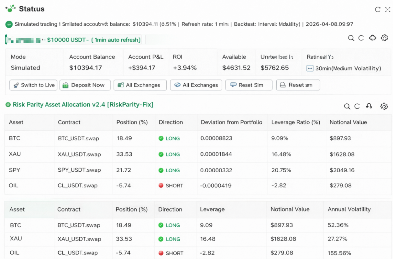
What It Looks Like Running Live

Once the strategy is running on the platform, the dashboard displays in real time whether each asset is currently long or short, its weight, the current leverage multiplier, the portfolio’s estimated annualized volatility, and the correlation matrix across the four assets. Floating P&L refreshes once per minute, and the strategy’s core calculations switch polling frequency automatically based on market volatility.

The 1-minute refresh isn’t achieved through multi-threading — it’s a nested sub-loop inside the main loop’s wait period, waking up every minute to fetch latest prices, update floating P&L, and update the equity curve. When the accumulated sleep time reaches the strategy’s polling interval, the sub-loop exits and the next strategy calculation cycle begins. The entire strategy is strictly single-threaded with no concurrency risk.

function sleepWithPnlRefresh(totalSleepMs, weights, leverage, covMatrix, corrMatrix) {
    var elapsed = 0;
    while (elapsed < totalSleepMs) {
        var step = Math.min(PNL_INTERVAL, totalSleepMs - elapsed);
        Sleep(step);
        elapsed += step;
        var prices = getTickers();
        var equity = calcEquity(prices);
        var initCap = _G('pt_initCapital') || INIT_CAPITAL;
        _chart.add(0, [new Date().getTime(), equity]);
        LogProfit(equity - initCap, '&');
        renderDashboard(weights, leverage, covMatrix, corrMatrix, prices, totalSleepMs, true);
    }
}

The strategy also supports a paper-trading mode, letting you run the full logic and debug parameters without committing real capital. Once behavior confirms expectations, you can evaluate whether to switch to live. With this configuration, paper trading ran for a stretch — here’s how it went.

Paper Trading Results

During the test period the strategy has been profitable overall for now. Position directions: BTC, XAU, and SPY all long; CL (crude) short. This happened to coincide with some easing in US–Iran tensions — geopolitical risk premium receded and crude prices fell quite visibly, and shorting crude was the main source of profit this round. The market movement during this period was friendly to the strategy — that doesn’t mean the future will be. In fact, there are still quite a few unresolved issues in the strategy itself, and not being upfront about them wouldn’t be honest.

Things I Haven’t Figured Out

Through building this strategy, a few issues are still open.

First, liquidity for RWA contracts is far below BTC’s. SPY, XAU, CL are still very new on-chain — slippage and order book depth are unknowns. Paper trading doesn’t surface this, but it will show up for real in live trading.

Second, the strategy relies on the assets maintaining some degree of non-correlation. But during periods of extreme market panic, correlations among risk assets tend to rise sharply, and the benefit of diversification gets eroded — precisely when you need protection most.

Third, traditional assets have non-trading hours where prices barely move, while BTC trades ²⁴⁄₇. This means the covariance matrix underestimates true co-movement — after US equities close, BTC keeps running, and the volatility during that window has no corresponding SPY data. When traditional markets reopen, the strategy’s view of co-movement may already be stale.

Fourth, historical data is limited, and the short-term stability of the covariance matrix is questionable. The EWMA decay coefficient, target volatility, and rebalance thresholds are all heuristic values without rigorous validation. The short-side judgment uses the sign of covariance with an equal-volatility reference portfolio — an engineering approximation. When multiple assets simultaneously have negative covariance with the reference portfolio, whether shorting them all genuinely reduces total portfolio risk needs to be verified individually and cannot simply be assumed. Crypto assets themselves have fat tails, and real return distributions deviate from normal — in extreme conditions the covariance matrix will underestimate risk. That’s a known bias you have to accept when working within the current framework.

Fifth, in live mode, during direction switches, after closing orders are sent the strategy waits a fixed duration and then proceeds to open new positions — without waiting for fill confirmation. If the exchange is slow to respond or there’s network latency, there’s a risk the old position isn’t fully closed before the new one opens. Paper trading doesn’t involve real fills so this isn’t visible — before going live, the wait duration should be evaluated against the specific exchange’s response time.

None of these issues can be uncovered by paper trading alone. They need more detailed modeling and theoretical work — every assumption has to be checked carefully before you can know whether this logic actually holds up in the crypto market.

Closing Thoughts

The motivation for building this strategy was simple: the crypto market is in a bear cycle, RWA contracts happen to fill out the major asset class picture, and traditional finance has decades of allocation theory. The two came together, and it was worth a try. The code is complete, the logic is transparent, the parameters are tunable. But this is ultimately just a starting point — there’s still a long way to go before it becomes an allocation strategy that genuinely stands up to live trading. If you have better ideas, let’s improve it together.

---

The content above only documents the exploration process of a strategy and does not constitute investment advice. Contract trading carries significant risk. Paper-trading performance doesn’t represent live results. Fully understand the risks before committing real capital.

Strategy source code: RWA Multi-Asset Risk Parity Strategy: https://www.fmz.com/m/edit-strategy/535843