[TOC]

I. Why Automated Factor Mining?

If you’ve been around quantitative trading, you’ve surely heard the word “factor.” What is a factor? Simply put, it’s a market signal expressed through data — price momentum, volume anomalies, Bollinger Band positioning — used to predict whether a given coin will go up or down over a certain period.

Sounds simple, but anyone who’s actually done factor research knows how hard it is:

• Solid financial knowledge and a deep background in mathematical statistics
• Large volumes of clean historical data
• A rigorous backtesting framework
• And an unavoidable problem: factor decay

A signal that works today might completely fail in a few days — because market participants learn, adapt, and arbitrage the pattern away. That’s why factor mining is never a one-time job; it requires continuous iteration.

What this article introduces is a system that automates this entire process: running a complete loop of factor mining → validation → elimination → signal synthesis → order execution at fixed intervals. Machine iteration replaces manual repetition, keeping the strategy in sync with the market’s evolving rhythm.

II. System Architecture Overview

The traditional factor mining workflow goes: researcher proposes hypothesis → writes code → runs backtest → filters → goes live → discovers it’s broken a few months later → starts over. The entire cycle can take weeks or even months.

This system compresses the entire loop into a single automated cycle executed at fixed intervals:

Step	Module	Description
Step 1	Get Symbol Pool	Filter high-liquidity perpetual contracts by trading volume; detect market state
Step 2	Check Factor Pool	Analyze current factor health; determine exploration direction for this round
Step 3	AI Factor Generation	Have AI generate new-dimension candidate factors within a constraint framework
Step 4	IC Validation	Replay historical data to compute Information Coefficient; eliminate ineffective factors
Step 5	Correlation Filtering & Culling	Remove information-overlapping factors; keep the factor pool lean and diverse
Step 6	Signal Synthesis & Execution	Weighted composite scoring; threshold-exceeding signals trigger rebalancing

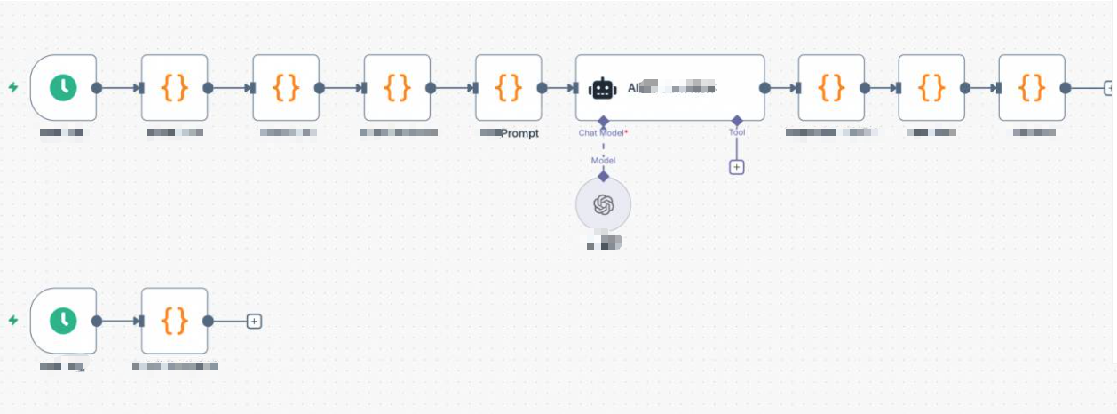
The system is driven by two schedulers: a slow trigger that executes the full factor iteration pipeline at hourly intervals, and a fast trigger that polls position status at second-level intervals, handling take-profit/stop-loss and dashboard refresh.

III. Module Details & Core Code

3.1 Get Symbol Pool

At the start of each round, the system pulls real-time quotes for all perpetual contracts from the exchange, sorted by trading volume to select the top N. Liquidity is a prerequisite for factor effectiveness — low-cap coins with sparse volume make any signal unreliable.

Simultaneously, it detects the BTC 4-hour candlestick volatility historical percentile to determine the overall market state (normal / high_vol / low_vol / volatile). This assessment directly influences the directional bias of AI-generated factors.

// Filter high-liquidity symbols by trading volume
const topN = $vars.topN || 150;
const tickers = exchange.GetTickers();
const filtered = tickers
    .filter(t => t.Symbol.endsWith('USDT.swap'))
    .map(t => ({ symbol: t.Symbol, quoteVolume: t.Last * t.Volume }))
    .sort((a, b) => b.quoteVolume - a.quoteVolume)
    .slice(0, topN)
    .map(t => t.symbol);
_G('afi_symbolPool', JSON.stringify(filtered));

// Detect BTC volatility percentile to determine market state
const btcR = exchange.GetRecords('BTC_USDT.swap', PERIOD_H4);
const n = btcR.length;
const returns20 = [];
for (let i = n - 20; i < n; i++)
    returns20.push(Math.abs((btcR[i].Close - btcR[i-1].Close) / btcR[i-1].Close));
const avgVol = returns20.reduce((a, b) => a + b, 0) / returns20.length;

// Compare against full-history volatility to determine percentile
const allVols = [];
for (let i = 1; i < n; i++)
    allVols.push(Math.abs((btcR[i].Close - btcR[i-1].Close) / btcR[i-1].Close));
allVols.sort((a, b) => a - b);
let btcVolPercentile = allVols.findIndex(v => v >= avgVol) / allVols.length;

let marketState = 'normal';
if (btcVolPercentile > 0.8) marketState = 'high_vol';
else if (btcVolPercentile < 0.3) marketState = 'low_vol';
_G('afi_marketState', marketState);
_G('afi_btcVolPct', btcVolPercentile.toFixed(2));

3.2 Check Factor Pool Status

Before asking AI to generate new factors, the system first takes stock of the current factor pool’s health: which factors have seen their recent IC consistently declining (decaying), and which dimensions haven’t been covered yet. This information is passed directly to the AI as constraints, preventing redundant exploration of already-failed directions.

const factorPool = JSON.parse(_G('afi_factorPool') || '[]');
const icHistory = JSON.parse(_G('afi_icHistory') || '{}');
const icDecayWindow = $vars.icDecayWindow || 48;       // Recent window length
const icDecayThreshold = $vars.icDecayThreshold || -0.01; // Decay threshold
const targetFactorCount = $vars.targetFactorCount || 10;

const degradedFactors = [];
for (const factor of factorPool) {
    const icArr = icHistory[factor.name] || [];
    if (icArr.length >= 20) {
        const window = Math.min(icArr.length, icDecayWindow);
        const recentAvg = icArr.slice(-window).reduce((a, b) => a + b, 0) / window;
        if (recentAvg < icDecayThreshold)
            degradedFactors.push({
                name: factor.name,
                recentIC: recentAvg.toFixed(4),
                rationale: factor.rationale
            });
    }
}

// Dynamically determine how many new factors to explore this round
const explorationBuffer = $vars.explorationBuffer || 3;
const explorationCount = Math.max(
    explorationBuffer,
    targetFactorCount - validCount + explorationBuffer
);
const action = factorPool.length === 0 ? 'generate_initial' : 'iterate_factors';

3.3 Build the Prompt: Let AI Invent Factors

What the AI receives is not an open-ended task, but a constrained framework. The prompt includes: current market state, list of currently effective factors (no duplicates allowed), recently decayed factors (no fine-tuning allowed), already-covered dimensions, and dimensions not yet explored.

This way, the candidate factors generated are genuine attempts in new directions, rather than re-running existing factors with tweaked parameters.

// Key snippet of the iteration-mode prompt
const usedDimensions = factorPool
    .map(f => f.name + '(' + (f.rationale || '') + ')')
    .join(', ') || 'None';

const validSummary = validFactors.map(f => {
    const arr = icHistory[f.name] || [];
    const avg = arr.length > 0
        ? (arr.reduce((a,b) => a+b, 0) / arr.length).toFixed(4) : 'N/A';
    const recent = arr.length >= 20
        ? (arr.slice(-20).reduce((a,b) => a+b, 0) / 20).toFixed(4) : 'N/A';
    return f.name + ': Historical IC=' + avg + ' Recent IC=' + recent
        + ' | Logic: ' + f.rationale;
}).join('\n') || 'None';

const degradedSummary = degradedFactors.length > 0
    ? degradedFactors.map(f =>
        f.name + ': Recent IC=' + f.recentIC + ' | Original logic: ' + f.rationale
    ).join('\n')
    : 'No decayed factors this round';

prompt += '【Currently Effective Factors (no variants needed)】\n' + validSummary + '\n\n';
prompt += '【Recently Decayed Factors (no fine-tuning on these dimensions)】\n' + degradedSummary + '\n\n';
prompt += '【Already Covered Dimensions (no duplicates)】\n' + usedDimensions + '\n\n';
prompt += '【Unexplored Dimensions (prioritize from here)】\n' + unusedSample + '\n\n';
prompt += 'Generate ' + explorationCount + ' entirely new-direction factors:\n';
prompt += '1. Must be completely different from covered dimensions; no fine-tuning of failed factors\n';
prompt += '2. Prioritize selection from unexplored dimensions\n';
prompt += '3. Prioritize designing nonlinear combination factors\n';
prompt += '4. Design for the current ' + marketState + ' market state\n';

The AI’s System Prompt includes a complete specification of the FMZ platform’s TA function library, code format constraints, crypto market prior knowledge, and a full list of explorable factor dimensions (see strategy source code for details). The output format is strictly pure JSON (no Markdown wrapping):

{
    "factors": [
        {
            "name": "MomentumAcceleration",
            "rationale": "Short-term momentum acceleration, capturing retail chase-rally inertia inflection points",
            "code": "(records[n-1].Close - records[n-6].Close)/records[n-6].Close - (records[n-2].Close - records[n-7].Close)/(records[n-7].Close + 0.0001)",
            "direction": 1,
            "type": "exploration"
        }
    ]
}

3.4 IC Validation: Let the Data Speak, Not Intuition

IC (Information Coefficient) measures how well the cross-sectional ranking derived from a factor correlates with the actual return ranking of the next candlestick. The higher the IC, the more accurate the factor’s prediction.

Validation uses historical walk-forward replay: taking several hundred past candlesticks, at each time point t, using the data from time t-1 to compute the factor value and predict the return of candlestick t. Time-series alignment is strict, eliminating any look-ahead bias.

function calcRankICFull(code, symRecords, factorName) {
    const syms = Object.keys(symRecords);
    const icList = [];
    const minLen = 30;
    const allLengths = syms.map(s => symRecords[s].length);
    const minSymLen = Math.min(...allLengths);
    const testLen = Math.min(500, minSymLen - 1);

    for (let t = minLen; t < testLen; t++) {
        const fVals = [], nRets = [];
        for (const sym of syms) {
            const fullRecords = symRecords[sym];
            // Use data up to t-1 to compute factor (slice(0, t) excludes candlestick t)
            const records = fullRecords.slice(0, t);
            const n = records.length;
            const v = (function() { return eval(code); })();
            if (isNaN(v) || !isFinite(v)) continue;
            fVals.push({ sym, val: v });
            // Predict the actual return of candlestick t
            nRets.push({
                sym,
                ret: (fullRecords[t].Close - fullRecords[t-1].Close) / fullRecords[t-1].Close
            });
        }
        if (fVals.length < 8) continue;

        // Compute Rank IC (Spearman correlation coefficient)
        const fRank = {}, rRank = {};
        [...fVals].sort((a,b) => a.val - b.val).forEach((x,i) => fRank[x.sym] = i);
        [...nRets].sort((a,b) => a.ret - b.ret).forEach((x,i) => rRank[x.sym] = i);

        const ss = fVals.map(x => x.sym);
        const fr = ss.map(s => fRank[s]);
        const rr = ss.map(s => rRank[s]);
        const n2 = ss.length;
        const fm = fr.reduce((a,b) => a+b, 0) / n2;
        const rm = rr.reduce((a,b) => a+b, 0) / n2;
        const num = fr.map((f,i) => (f-fm) * (rr[i]-rm)).reduce((a,b) => a+b, 0);
        const den = Math.sqrt(
            fr.map(f => (f-fm)**2).reduce((a,b) => a+b, 0) *
            rr.map(r => (r-rm)**2).reduce((a,b) => a+b, 0)
        );
        if (den > 0) icList.push(num / den);
    }
    const avgIC = icList.length > 0
        ? icList.reduce((a,b) => a+b, 0) / icList.length : 0;
    return { avgIC, icList };
}

The IC threshold is controlled by the variable $vars.icThreshold, defaulting to 0.02. This is a relatively lenient entry-level threshold, suitable for quickly filtering out obviously ineffective factors. For stricter statistical significance control, this value can be raised according to actual needs. Factors that fail to pass the threshold are eliminated regardless of how perfect their logic may be.

3.5 Correlation Filtering & Bottom Culling

Factors that pass IC validation still need to clear two more hurdles:

First hurdle: Correlation filtering. If two factors have highly similar cross-sectional scores (|corr| > threshold), keep the one with higher IC and discard the other. When two factors are highly correlated in their cross-sectional scores, they are essentially capturing nearly identical information — keeping one is sufficient; adding another doesn’t add a new perspective.

Second hurdle: Bottom culling. The factor pool has a capacity limit; excess factors are ranked by performance, and the worst ones are eliminated. Factors with recently declining IC are ranked using their recent IC rather than historical average IC, subjecting them to greater elimination pressure.

// Correlation filtering (keep highest IC, discard highly correlated redundant factors)
const corrThreshold = $vars.corrThreshold || 0.7;
survivedFactors.sort((a, b) => b.icAvg - a.icAvg); // Sort by IC descending first

const decorrelatedFactors = [];
for (const factor of survivedFactors) {
    let isRedundant = false;
    for (const selected of decorrelatedFactors) {
        const corr = Math.abs(calcCorrelation(
            factorScoresMap[factor.name],
            factorScoresMap[selected.name]
        ));
        if (corr > corrThreshold) {
            // Record absorbed correlated factor (for dashboard display)
            selected.corrGroup = (selected.corrGroup ? selected.corrGroup + ',' : '')
                + factor.name;
            isRedundant = true;
            break;
        }
    }
    if (!isRedundant) decorrelatedFactors.push({ ...factor, corrGroup: '' });
}

// Bottom culling: decaying factors ranked by recent IC instead of historical average
const targetFactorCount = $vars.targetFactorCount || 10;
decorrelatedFactors.sort((a, b) => {
    const scoreA = a.isDecaying ? a.recentIC : a.icAvg;
    const scoreB = b.isDecaying ? b.recentIC : b.icAvg;
    return scoreB - scoreA;
});
const finalPool = decorrelatedFactors.slice(0, targetFactorCount);
_G('afi_factorPool', JSON.stringify(finalPool));

Note: The correlation calculation is based on factor scores from the current cross-section, which may produce occasional misjudgments at certain points in time. A more robust approach would be to average correlations across multiple historical cross-sections — this is a direction for future improvement.

3.6 Signal Synthesis & Rebalancing Execution

Once the factor pool is stable, the system computes a composite score for each symbol: Z-score standardize each factor’s cross-sectional values, then combine them with weighted summation based on each factor’s recent IC — better-performing factors get larger weight, and factors with negative recent IC have their weight set to zero.

// Factor weights: recent IC weighted (negative IC factors get zero weight)
const weights = {};
let totalW = 0;
for (const f of factorPool) {
    const arr = icHistory[f.name] || [];
    const recentArr = arr.slice(-48);
    const recentIC = recentArr.length > 0
        ? recentArr.reduce((a,b) => a+b, 0) / recentArr.length : 0;
    const w = Math.max(0, recentIC); // Negative IC → weight = 0
    weights[f.name] = w;
    totalW += w;
}
if (totalW > 0) Object.keys(weights).forEach(k => weights[k] /= totalW);
else factorPool.forEach(f => weights[f.name] = 1 / factorPool.length);

// Z-score standardization
function zscore(fname) {
    const vals = validSyms
        .map(s => ({ sym: s, val: rawMatrix[s][fname] }))
        .filter(x => x.val !== null);
    if (vals.length < 5) return {};
    const mean = vals.reduce((a,b) => a + b.val, 0) / vals.length;
    const std = Math.sqrt(vals.reduce((a,b) => a + (b.val - mean)**2, 0) / vals.length);
    const r = {};
    vals.forEach(x => r[x.sym] = std > 0 ? (x.val - mean) / std : 0);
    return r;
}

// Composite scoring
const scores = {};
for (const sym of validSyms) {
    let score = 0;
    for (const f of factorPool) {
        const z = zscore(f.name)[sym];
        if (z !== undefined) score += weights[f.name] * f.direction * z;
    }
    scores[sym] = score;
}

// Threshold filtering: skip ambiguous signals, don't enter positions
const longShortN = $vars.longShortN || 5;
const longThreshold = $vars.longThreshold || 0.3;
const shortThreshold = $vars.shortThreshold || -0.3;

const sorted = Object.keys(scores).sort((a,b) => scores[b] - scores[a]);
const longList = sorted.filter(s => scores[s] >= longThreshold).slice(0, longShortN);
const shortList = sorted.slice().reverse()
    .filter(s => scores[s] <= shortThreshold).slice(0, longShortN);

During rebalancing execution, old positions not in the current round’s list are closed first, then new signals are entered proportionally based on account equity:

const positionRatio = $vars.positionRatio || 0.8; // Total equity usage ratio
const maxLeverage = $vars.maxLeverage || 3;
const account = exchange.GetAccount();
const equity = account.Equity || account.Balance;
const perAmt = (equity * positionRatio) / (longList.length + shortList.length);

// Close old positions not in the target set
const targetSet = new Set([...longList, ...shortList]);
for (const sym of Object.keys(currentHoldings)) {
    if (!targetSet.has(sym)) {
        const pos = currentHoldings[sym];
        const isLong = pos.Type === PD_LONG || pos.Type === 0;
        exchange.CreateOrder(sym,
            isLong ? 'closebuy' : 'closesell', -1, Math.abs(pos.Amount));
        // Clear take-profit tracking state
        const cm = sym.match(/^(.+)_USDT/);
        if (cm) {
            _G(cm[1] + '_maxpnl', null);
            _G(cm[1] + '_trail', null);
        }
    }
}

// Enter new signal positions (using market orders, -1 indicates market price)
function openPos(sym, isLong) {
    exchange.SetMarginLevel(sym, maxLeverage);
    const market = allMarkets[sym];
    const price = exchange.GetTicker(sym).Last;
    const ctVal = (market.CtVal && market.CtVal > 0) ? market.CtVal : 1;
    const amtPrec = market.AmountPrecision !== undefined ? market.AmountPrecision : 0;
    const minQty = (market.MinQty && market.MinQty > 0) ? market.MinQty : 1;
    const maxQty = (market.MaxQty && market.MaxQty > 0) ? market.MaxQty : 999999;
    let qty = _N(perAmt / price / ctVal, amtPrec);
    qty = Math.min(Math.max(qty, minQty), maxQty);
    exchange.CreateOrder(sym, isLong ? 'buy' : 'sell', -1, qty);
}

3.7 Position Monitoring: Stop-Loss / Take-Profit / Dynamic Trailing Stop

The fast trigger runs at second-level intervals, monitoring the unrealized P&L of all positions in real time and executing three exit strategies:

• Fixed stop-loss: Auto-close when unrealized loss exceeds STOP_LOSS_PCT (default 5%)
• Fixed take-profit: Auto-close when unrealized profit exceeds TAKE_PROFIT_PCT (default 10%)
• Dynamic trailing stop: Activated once unrealized profit reaches TRAIL_TRIGGER (3%); the drawdown threshold adjusts dynamically with the peak unrealized profit

const STOP_LOSS_PCT = $vars.stopLossPct || 5;
const TAKE_PROFIT_PCT = $vars.takeProfitPct || 10;
const TRAIL_TRIGGER = 3; // Activate trailing stop after 3% unrealized profit

// Dynamic drawdown threshold: higher peak profit allows larger drawdown
function getDynamicTrailDrawdown(maxPnl) {
    if (maxPnl >= 7) return 3;   // Peak profit ≥7%, allow 3% drawdown
    if (maxPnl >= 4) return 2;   // Peak profit ≥4%, allow 2% drawdown
    return 1.5;                   // Otherwise, 1.5% drawdown
}

function monitorTPSL(positions, tickers) {
    for (const pos of (positions || [])) {
        if (Math.abs(pos.Amount) === 0) continue;
        const cm = pos.Symbol.match(/^(.+)_USDT/);
        if (!cm) continue;
        const coin = cm[1];
        const ticker = tickers[coin + '_USDT.swap'];
        if (!ticker) continue;

        const isLong = pos.Type === PD_LONG || pos.Type === 0;
        const cur = ticker.Last;
        const ent = pos.Price;
        const amt = Math.abs(pos.Amount);
        const pnlPct = (cur - ent) * (isLong ? 1 : -1) / ent * 100;

        // Track peak unrealized profit
        let maxPnl = _G(coin + '_maxpnl');
        if (maxPnl === null) {
            maxPnl = pnlPct;
            _G(coin + '_maxpnl', maxPnl);
        } else if (pnlPct > maxPnl) {
            maxPnl = pnlPct;
            _G(coin + '_maxpnl', maxPnl);
        }

        // Activate trailing stop
        if (!_G(coin + '_trail') && maxPnl >= TRAIL_TRIGGER) {
            _G(coin + '_trail', true);
            Log(coin + ' trailing stop activated, unrealized profit: +'
                + pnlPct.toFixed(2) + '%');
        }

        const trailDrawdown = getDynamicTrailDrawdown(maxPnl);

        let reason = null;
        if (_G(coin + '_trail') && (maxPnl - pnlPct) >= trailDrawdown)
            reason = 'Trailing stop (drawdown ' + (maxPnl - pnlPct).toFixed(2)
                + '%, threshold ' + trailDrawdown + '%)';
        if (!reason && pnlPct <= -STOP_LOSS_PCT)
            reason = 'Stop-loss (' + pnlPct.toFixed(2) + '%)';
        if (!reason && pnlPct >= TAKE_PROFIT_PCT)
            reason = 'Take-profit (' + pnlPct.toFixed(2) + '%)';

        if (reason) {
            exchange.CreateOrder(pos.Symbol,
                isLong ? 'closebuy' : 'closesell', -1, amt);
            Log(coin, 'triggered', reason);
            _G(coin + '_maxpnl', null);
            _G(coin + '_trail', null);
        }
    }
}

IV. Key Design Decisions

4.1 Why Rank IC (Instead of Pearson IC)

Rank IC computes correlation using ranks rather than raw values, making it naturally robust against extreme values (outliers). The crypto market has heavily fat-tailed price distributions. Pearson IC is easily distorted by a handful of extreme candlesticks, while Rank IC offers greater stability.

4.2 Strict Time-Series Alignment: Eliminating Look-Ahead Bias

Both IC validation and live signal computation uniformly use t-1 period factor values to predict t-period returns. During validation, records are passed as fullRecords.slice(0, t), physically truncating future data so that no matter how AI-generated factor code references records[n], it can only access history up to t-1. In live mode, the last candlestick is removed (slice(0, n-1)) before computing factor values to predict the next candlestick’s movement. The logic is identical in both cases, preventing inflated IC from look-ahead data leakage.

4.3 Recent IC Weighting: Weights Self-Adapt to the Market

Factor weights are not fixed but dynamically adjusted based on recent IC. When a factor starts failing (recent IC declining), its weight in signal synthesis automatically decreases toward zero. The system completes weight rebalancing without any manual intervention.

4.4 Dual-Trigger Architecture

Factor iteration is a computationally heavy task (candlestick fetching + IC backtesting + AI calls) — running it at hourly intervals is sufficient. Position protection is a time-sensitive task requiring second-level response. Splitting these into triggers with different frequencies prevents them from blocking each other.

V. Live Observations: The Factor Iteration Process

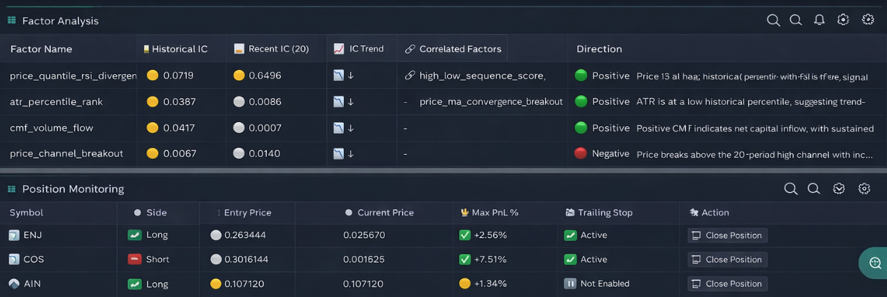
After two days of live operation, the following phenomena were observed:

• Factors that entered the pool early generally had historical ICs between 0.04 and 0.07, passing the basic threshold.
• As iterations progressed, nearly all factors saw their recent IC declining — some dropping from 0.06 to 0.008, others falling into negative territory. This indicates that the signals these factors captured are becoming ineffective in the current market environment.
• After the system detected decay, the next round prioritized exploring uncovered dimensions, searching for new candidate factors as replacements. The entire process required no manual intervention.

Two days is too short to sufficiently validate whether the system’s self-adaptive capability is genuinely effective. This section merely documents that the system executed the iteration actions as designed. More meaningful conclusions require longer-term sustained observation. However, this process itself already demonstrates that the system’s fundamental design logic is functioning: it doesn’t stubbornly cling to failed signals, but continuously attempts new dimensions.

VI. Closing Thoughts

Building this system wasn’t about proving that AI can beat the market. Rather, it’s about showing that in the age of AI, many things that only top-tier institutions could previously accomplish are now within reach for ordinary individuals to attempt.

Factor mining, strategy iteration, automated execution — these things that used to require a team, massive data infrastructure, and years of accumulation to build, can now be run as a single workflow.

This doesn’t mean it will produce consistent profits. The market is always more complex than any system. But it does mean that the barrier to entry is lowering, the tools are getting stronger, and the possibility for ordinary people to participate in this endeavor is growing.

⚠️ Risk Disclaimer: All strategies carry the risk of losses. The content of this article is for technical learning purposes only and does not constitute investment advice. Please test thoroughly before going live.

Strategy Source Code: Adaptive Factor Mining Quantitative Strategy (Test Version)