From 99 Traders to One Signal: Implementing a Distilled KOL Consensus Strategy on FMZ

The word “distillation” has been showing up everywhere lately. In AI it usually means compressing complex capabilities into a more compact, reusable form. The same idea carries over to strategy research — and when you make it concrete, what you’re really doing is taking knowledge that was previously scattered, fuzzy, and dependent on subjective experience, and turning it into something you can compute, verify, and continue to refine.

The crypto-kol-quant project has been getting a lot of attention recently. What’s actually interesting about it isn’t the number of KOLs it scrapes, or the fact that it uses LLMs. It’s that the project tries to do something quantitative research rarely attempts: distill traders’ experience into a set of computable capability factors, and then aggregate those factors into a consensus signal. That’s a question worth taking seriously. Because if a group of long-active, stylistically consistent traders really have built up their own cognitive frameworks for the market, those frameworks shouldn’t only live in tweets, charts, and offhand remarks — they ought to be extractable, organized, and made part of a runnable strategy pipeline.

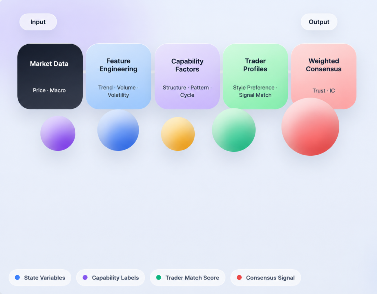
Working from that premise, we built an early implementation inside the FMZ environment. The goal wasn’t to “port” the project — it was to wire up its core logic from end to end: pull market data, translate the market into structured state, decide which trading capabilities are being triggered by that state, map those capabilities back to trader profiles, and finally aggregate every trader’s individual judgment into a weighted consensus signal. It’s clearly not a finished trading system, but it does demonstrate one important thing: trader experience really can be compressed, structured, and inserted into a strategy’s decision flow.

What Gets Distilled Is Capability, Not Opinion

When people first encounter a project like this, they tend to read it as “a KOL sentiment strategy.” That’s not quite right. The original project isn’t trying to count who’s bullish today or who’s calling tops and bottoms. It’s pushing further: how does this trader actually understand the market? Under what kind of structure does he lean long? Does he focus on trend, position, pattern, volatility, or macro context? And can the way he makes those calls be organized into a stable set of capability tags?

Once you frame the problem that way, the strategy’s center of gravity shifts. The system stops caring about any single statement and starts caring about the methodology behind it. Put differently: what gets distilled here isn’t text — it’s trading knowledge itself. The system tries to translate subjective experience, which used to require a human to interpret, into rules a program can recognize and call. That’s the biggest difference between this and the usual sentiment models. It’s not measuring how hot the market mood is. It’s reconstructing how different trading frameworks would react to the current market.

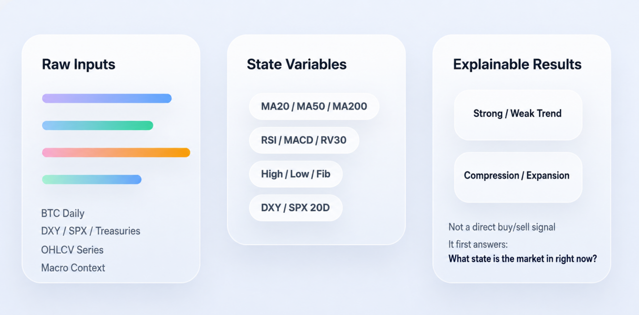
Step 1: Translate the Market Into State Variables

For distillation to actually land, the first step can’t be prediction — it has to be feature engineering. The reason is simple: a trader’s language is written for humans, not programs. Take a sentence like “price pulled back to a key moving average, decent spot to add on the second tap.” A trader gets it instantly, but a program has to break it down: which moving average — the 50-day or the 200-day? Is price actually near that line? Is the trend still intact? Did a confirming candle appear?

So the system’s first job isn’t to produce a long/short call. It’s to convert raw market data into a set of structured states. The most basic layer here uses price to build trend and momentum features. Moving averages, exponential moving averages, RSI, MACD — these aren’t there to pile up indicators, they’re there to answer a simple question: roughly what state is the market in right now?

The key code:

# Use moving averages of different periods to describe price's position within trends
f['ma20']  = _sma(c, 20)
f['ma50']  = _sma(c, 50)
f['ma100'] = _sma(c, 100)
f['ma200'] = _sma(c, 200)

# Exponential moving averages weight recent price changes more heavily
f['ema20'] = _ema(c, 20)
f['ema50'] = _ema(c, 50)

# RSI captures whether the market is overbought/oversold or losing momentum
f['rsi14'] = _rsi(c, 14)

# MACD line, signal line, and histogram together track trend and momentum shifts
ml, ms, mh = _macd(c)
f['macd']      = ml
f['macd_sig']  = ms
f['macd_hist'] = mh

The code isn’t doing anything complicated. Moving averages help the system locate current price relative to longer-term trend; RSI and MACD describe whether momentum is building or fading. None of this is a trading decision yet — it’s purely a “market state” layer.

The system also adds volatility and positional features, because a lot of trading judgments don’t rely on trend alone — they also depend on whether we’re in a volatility-compression phase, or whether price is sitting near a range high or low.

The corresponding code:

# Log returns are the basis for volatility computation
logr = np.log(c / c.shift(1))

# 30-day annualized realized volatility, gauging current volatility level
# Note: sqrt(365) — crypto trades around the clock, so we annualize on
# calendar days rather than the 252 trading days used for equities
f['rv30'] = logr.rolling(30, min_periods=10).std() * np.sqrt(365)

# Recent 20-day and 50-day highs/lows, used to locate price within recent structure
f['high_20d'] = h.rolling(20, min_periods=1).max()
f['low_20d']  = l.rolling(20, min_periods=1).min()
f['high_50d'] = h.rolling(50, min_periods=1).max()
f['low_50d']  = l.rolling(50, min_periods=1).min()

rv30 captures the recent annualized volatility level. The range highs/lows tell the system where current price sits inside the recent price structure. On top of that, macro context gets folded into the state space too — there’s a kind of trader who doesn’t only look at the coin price; they’re simultaneously watching the dollar index, equity risk appetite, and the rate environment. The code aligns these to the daily frame and then turns them into readable state:

# DXY as a backdrop for dollar strength
if 'DXY' in macro:
    dxy = _align(macro['DXY'])
    f['dxy_ret_20d']    = dxy.pct_change(20)
    f['dxy_trend_down'] = (dxy.pct_change(20) < -0.01).astype(int)

# SPX as a proxy for risk appetite
if 'SPX' in macro:
    spx = _align(macro['SPX'])
    f['spx_ret_20d']  = spx.pct_change(20)
    f['spx_trend_up'] = (spx.pct_change(20) > 0).astype(int)

The point of this whole step compresses to one sentence: take “what the market looks like right now” and turn it into structured state the machine can keep reading. Without this layer, there’s nothing left to distill.

Step 2: Encode Subjective Experience as Capability Factors

Features alone aren’t enough — features only describe the market, they don’t say what that state means. The next step is to write traders’ experience into rules: given the current state variables, decide which trading capabilities are being triggered.

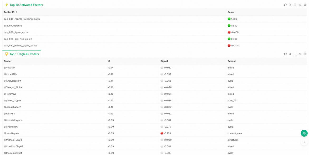
This is where the strategy’s distillation flavor is strongest. We’re no longer talking abstractly about “frameworks that matter”; we’re committing them to actual program conditions. The current implementation’s capability factors span pattern, structure, indicator, cycle, and macro layers. Some come from pattern recognition — bull flags, bear flags, double tops/bottoms, head-and-shoulders, triangles. Some come from structural analysis — Wyckoff, SMC, ICT-style frameworks. Some come from indicators themselves — RSI divergences, golden/death crosses, Bollinger band squeeze breakouts. And some come from cycle and macro context — halving cycles, trending vs. ranging market regime shifts, DXY drawdowns, risk-on rebounds.

A textbook example is “trend pullback continuation.” Plenty of traders share this pattern: if the larger trend is still up, price pulls back to a key moving average, and the current candle shows a confirming bid, that often means the trend continues. The program states it directly:

# Check whether current price is close to the 50-day moving average
near_ma50 = abs(close - ma50_v) / close < 0.02 if close > 0 else False

# If the 50-day MA is still above the 200-day MA, and a green candle shows up
# right at the pullback, score this as a trend-continuation capability signal
# (In production you'd want extra confirmation — volume, candle body, lower wick)
s['cap_014_trend_pullback_continuation'] = 0.6 if (ma50_gt and near_ma50 and is_green) else 0.0

There’s nothing mysterious here — it’s just breaking a sentence of human language into a few conditions a machine can evaluate one by one. Another example is “Bollinger squeeze breakout.” For many traders, a long stretch of compressed volatility followed by a sudden expansion (up or down) usually signals a fresh directional choice. The rule looks like:

# bb_w20_p1 is the 20-period mean of Bollinger bandwidth (the squeeze baseline).
# If the previous candle's bandwidth sits below that baseline, treat it
# as a volatility-contraction state.
squeezed = bb_w_p1 < bb_w20_p1 if bb_w20_p1 > 0 else False

# Squeeze followed by a breakout above the upper band -> positive signal
# Squeeze followed by a break below the lower band  -> negative signal
s['cap_021_bollinger_squeeze_breakout'] = (
    0.6  if (squeezed and close > bb_u) else
   -0.6  if (squeezed and close < bb_l) else 0.0
)

Macro factors get the same treatment. For traders who lean macro, BTC isn’t an isolated price series — it’s affected by the dollar, equities, and the rate environment, so those views are also written into capability checks:

# Falling DXY is generally read as a positive backdrop for BTC
s['cap_027_dxy_inverse_btc']  = 0.4 if (not _nm(dxy_r20) and dxy_r20 < -0.01) else 0.0

# Rising S&P implies improving risk appetite
s['cap_028_spx_risk_on_off']  = 0.4 if (not _nm(spx_r20) and spx_r20 >  0.02) else 0.0

# Falling short-end yields imply a marginal liquidity tailwind
s['cap_029_yields_liquidity'] = 0.4 if (not _nm(y_r20)   and y_r20   < -0.02) else 0.0

What matters at this layer isn’t how many rules we wrote — it’s that we completed the most critical move in the entire distillation: compressing judgments that previously required subjective interpretation into computable conditions. Worth noting in passing: most capability factors in the current version are condition-triggered rather than continuously scored. That means the system is closer to detecting whether a particular structure holds than to repricing every micro-fluctuation. It’s why this implementation fits daily or mid-to-low frequency reasoning better than high-frequency trading.

Step 3: Don’t Sum Factors — Map Them Back to Trader Profiles

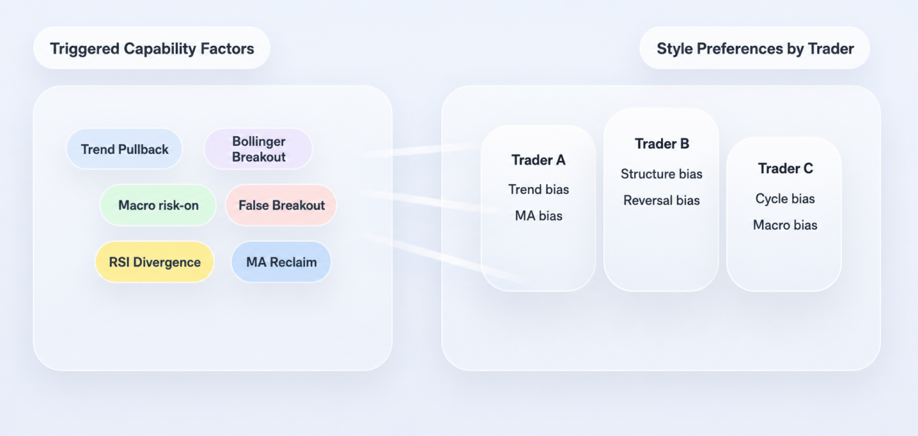
If the strategy stopped at the factor layer, it would still just be a regular rule system. What makes the original project distinctive is that it doesn’t stop there — it pushes one step further: factors don’t directly determine direction; they get mapped back to trader profiles first.

This part matters. Real traders don’t “use all capabilities equally.” Some lean into trend, some into structure, some into cycle, some into macro. Faced with the same market state, different traders care about completely different things. So instead of averaging all factors at once, the system reads each trader’s capability preferences first, then computes that trader’s individual signal given the current factor state.

The profile-loading logic:

# For each trader, load the capability factors they actually use, with weights
caps = {c['id']: float(c.get('weight', 0.5))
        for c in p.get('capabilities_used', [])}

profiles.append({
    'handle': p.get('handle', item['name'][:-5]),
    'caps':   caps
})

Each profile is essentially answering one question: which capability factors does this trader actually rely on, and how heavily does each one weigh in his framework? Once profiles are in hand, the system computes each trader’s “personal signal” for the current market:

for p in profiles:
    sig = 0.0
    wt  = 0.0

    # Iterate over every capability this trader cares about
    for cap_id, w in p['caps'].items():
        score = factor_scores.get(cap_id, 0.0)

        # Current factor score scaled by this trader's preference weight
        sig += w * score
        wt  += abs(w)

    # Normalize to get this trader's personal signal in the current market
    trader_raw = sig / wt if wt > 0 else 0.0

By this point the system feels different. It’s no longer just looking at “which factors lit up.” It’s approximating something else: if you handed today’s market to these 99 traders, how would each of them judge it?

Step 4: From Personal Signals to Weighted Consensus

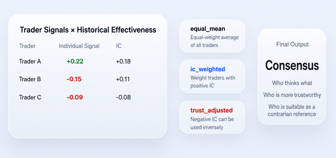
Once each trader’s personal signal is computed, the system finally enters the consensus layer. “Consensus” here isn’t a vote, and it’s definitely not whoever-shouts-loudest-wins — it factors in historical effectiveness as well.

A quick note for readers new to the term: IC stands for Information Coefficient — the historical correlation between a signal and forward returns. Higher absolute IC means the signal carries more information.

The two most important outputs in the current code are ic_weighted and trust_adjusted. The core logic:

# First: weight only traders with positive IC, producing ic_weighted
pos_w  = sum(max(t['ic'], 0) for t in trader_signals)
ic_wt  = (
    sum(t['signal'] * max(t['ic'], 0) for t in trader_signals) / pos_w
    if pos_w > 0 else 0.0
)

# trust_adjusted goes a step further:
# positive-IC traders are used directly; negative-IC traders are flipped
# and then everything is weighted by absolute IC magnitude
abs_w = sum(abs(t['ic']) for t in trader_signals)
trust = (
    sum((t['signal'] if t['ic'] >= 0 else -t['signal']) * abs(t['ic'])
        for t in trader_signals) / abs_w
    if abs_w > 0 else 0.0
)

Two simple but important principles are embedded here. First: traders who’ve been more effective historically carry more weight today. Second: traders whose historical IC is negative aren’t thrown out — they may be used as inverse indicators instead. So trust_adjusted isn’t just “what does the crowd think” — it’s “who thinks what, and whose view do we actually trust.”

One caveat worth flagging: flipping a negative-IC trader assumes that negative IC reflects stable contrarian information, not statistical noise. In practice you’d want a significance test or a sample-size gate before using the inverse — otherwise you’re amplifying randomness instead of correcting it.

This is also why the system reads differently from a normal sentiment model. It isn’t tallying voices — it’s running a round of cognitive aggregation that’s been checked against history. Compress the whole method into one sentence: turn the market into state variables, map state variables into capability factors, map capability factors into per-trader personal signals, and finally aggregate those personal signals by historical effectiveness into a consensus call.

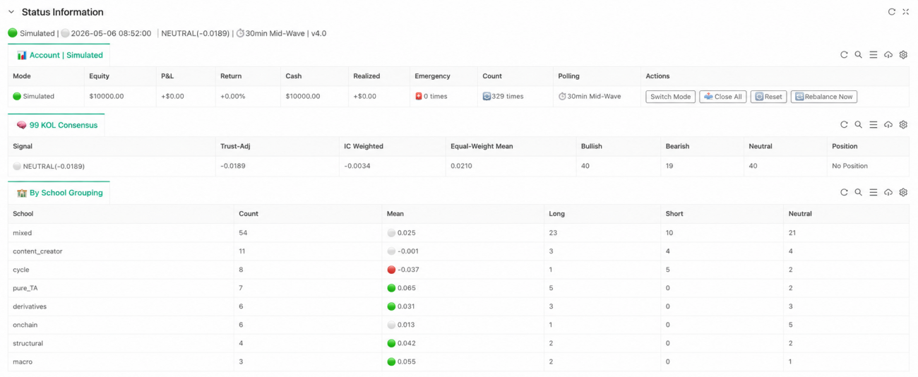
What the FMZ Implementation Actually Achieves

If the project stayed in research mode, the system would feel more like a “consensus analyzer.” On FMZ, the priority is wiring the entire pipeline so it can keep running. The most important code is just three lines:

# Step 1: turn raw price data and macro variables into structured state
feat_df = build_features(records, macro if macro else None)

# Step 2: evaluate which capability factors are triggered given the state
factor_scores = evaluate_factors(feat_df)

# Step 3: map factors back to trader profiles, then aggregate to consensus
consensus = compute_consensus(factor_scores)

These three lines are the strategy’s three most important abstractions. Layer one handles market state; layer two handles capability evaluation; layer three handles trader consensus. Execution, risk control, and state display sit downstream of these, but from a research-logic perspective the critical part is already complete. The point of this implementation isn’t how many runtime details it adds — it’s that the original project’s capability profiles are no longer static files, the factors are no longer just research outputs, and the consensus is no longer just a number in a report. They’ve been wired into a continuously running judgment loop.

Why It’s Still Just a Prototype

This implementation isn’t the endgame. The current code uses BTC daily bars, so it’s better suited to mid-to-low frequency consensus calls than to high-frequency trading. Its core still revolves around daily structure, cycle position, macro backdrop, and trader capability preferences. Trader profiles and IC values are still static inputs — the system hasn’t yet entered an online-evolution phase. In other words, “knowledge distillation” step one is done, but “the distilled knowledge keeps self-correcting” hasn’t fully landed.

That doesn’t take away from what the project does demonstrate, which is itself important: trader experience really can be compressed, structured, and inserted into a strategy pipeline. The value isn’t that it produces stable returns yet — it’s that it advances a research path that previously sat at the concept level into something runnable. How those capability factors should evolve, how trader weights should update, and how consensus should keep recalibrating against live markets — those are questions only more runtime data can answer.

Closing

What’s genuinely instructive about crypto-kol-quant isn’t the volume of trendy concepts it strings together. It’s that it pushes a hard-to-systematize problem one step forward: take traders’ experience, turn it from expression into capabilities, from capabilities into factors, from factors into consensus. The FMZ implementation’s job is to actually run that distillation pipeline end-to-end. It doesn’t oversell itself as the final answer, and it doesn’t try to hide the fact that it’s still an early prototype. But it does prove one thing: trading experience doesn’t have to live only in charts and language — it can be distilled, structured, executed, and even placed inside a system that continuously judges the market.

If traditional quant is good at finding patterns inside price series, then a strategy of this kind points to a direction worth pushing: extract patterns from human cognition, then let those patterns participate in the market in turn. And that, more than anything else, may be why “distillation” deserves attention in strategy research.

---

Original project: Tower of Locked Demons Skill — Refining 99 Crypto Traders (suo yao ta Skill)

Special thanks to user GiantBin for the underlying ideas. If you have your own thoughts on this direction, we’d welcome the conversation.