

Neural Networks and Digital Currency Quantitative Trading Series (2) - Intensive Learning and Training Bitcoin Trading Strategy
1. Introduction
In the last article, we introduced the use of LSTM network to predict the price of Bitcoin: https://www.fmz.com/bbs-topic/9879, as mentioned in the article, it is only a small training project to familiarize with RNN and pytorch. This article will introduce the use of intensive learning to train the trading strategies directly. The model of intensive learning is OpenAI open source PPO, and the environment refers to the style of gym. In order to facilitate understanding and testing, the PPO model of LSTM and the gym environment for backtesting are written directly without using ready-made packages.
PPO, or Proximal Policy Optimization, is an optimization improvement of Policy Gradient. gym was also released by OpenAI. It can interact with the strategy network and feedback the status and rewards of the current environment. It is like the practice of intensive learning. It uses the PPO model of LSTM to make instructions, such as buying, selling or no operation directly according to the market information of Bitcoin. The feedback is given by the backtest environment. Through training, the model is optimized continuously to achieve the goal of strategic profit.
Reading this article requires a certain foundation of in-depth intensive learning in Python, pytorch and DRL. But it doesn't matter if you can't. It's easy to learn and get started with the code given in this article. This tutorial is produced by the FMZ Quant Trading platform (www.fmz.com). Welcome to join the QQ group: 863946592 for communication.
2. Data and learning references
Bitcoin price data sourced from FMZ Quant Trading platform: https://www.quantinfo.com/Tools/View/4.html.
An article using DRL+gym to train trading strategies: https://towardsdatascience.com/visualizing-stock-trading-agents-using-matplotlib-and-gym-584c992bc6d4.
Some examples of getting started with pytorch: https://github.com/yunjey/pytorch-tutorial.
This article will implement by the LSTM-PPO model directly: https://github.com/seungeunrho/minimalRL/blob/master/ppo-lstm.py.
Articles about PPO: https://zhuanlan.zhihu.com/p/38185553.
More articles about DRL: https://www.zhihu.com/people/flood-sung/posts.
About gym, this article does not require installation, but it's very common in intensive learning: https://gym.openai.com/.
3. LSTM-PPO
For an in-depth explanation of PPO, you can learn from the previous reference materials. Here is just a simple introduction to concepts. The last issue of the LSTM network only predicted the price. How to buy and sell based on the predicted price will have to be realized separately. It is natural to think that the direct output of the trading action will be more direct. This is the case with Policy Gradient, which can give the probability of various actions according to the input environment information s. The loss of LSTM is the difference between the predicted price and the actual price, while the loss of PG is - log (p) * Q, where p is the probability of an output action, and Q is the value of the action (such as reward score). The intuitive explanation is that if the value of an action is higher, the network should output a higher probability to reduce the loss. Although PPO is much more complex, its principle is similar. The key is how to better evaluate the value of each action and how to better update parameters.
The source code of LSTM-PPO is given below, which can be understood in combination with the previous data:
import time
import requests
import json
import numpy as np
import pandas as pd
import torch
import torch.nn as nn
import torch.nn.functional as F
import torch.optim as optim
from torch.distributions import Categorical
from itertools import count
# Hyperparameters of the model
learning_rate = 0.0005
gamma = 0.98
lmbda = 0.95
eps_clip = 0.1
K_epoch = 3
device = torch.device('cpu') # It can also be changed to GPU version.
class PPO(nn.Module):
def __init__(self, state_size, action_size):
super(PPO, self).__init__()
self.data = []
self.fc1 = nn.Linear(state_size,10)
self.lstm = nn.LSTM(10,10)
self.fc_pi = nn.Linear(10,action_size)
self.fc_v = nn.Linear(10,1)
self.optimizer = optim.Adam(self.parameters(), lr=learning_rate)
def pi(self, x, hidden):
# Output the probability of each action. Since LSTM network also contains the information of hidden layer, please refer to the previous article.
x = F.relu(self.fc1(x))
x = x.view(-1, 1, 10)
x, lstm_hidden = self.lstm(x, hidden)
x = self.fc_pi(x)
prob = F.softmax(x, dim=2)
return prob, lstm_hidden
def v(self, x, hidden):
# Value function is used to evaluate the current situation, so there is only one output.
x = F.relu(self.fc1(x))
x = x.view(-1, 1, 10)
x, lstm_hidden = self.lstm(x, hidden)
v = self.fc_v(x)
return v
def put_data(self, transition):
self.data.append(transition)
def make_batch(self):
# Prepare the training data.
s_lst, a_lst, r_lst, s_prime_lst, prob_a_lst, hidden_lst, done_lst = [], [], [], [], [], [], []
for transition in self.data:
s, a, r, s_prime, prob_a, hidden, done = transition
s_lst.append(s)
a_lst.append([a])
r_lst.append([r])
s_prime_lst.append(s_prime)
prob_a_lst.append([prob_a])
hidden_lst.append(hidden)
done_mask = 0 if done else 1
done_lst.append([done_mask])
s,a,r,s_prime,done_mask,prob_a = torch.tensor(s_lst, dtype=torch.float), torch.tensor(a_lst), \
torch.tensor(r_lst), torch.tensor(s_prime_lst, dtype=torch.float), \
torch.tensor(done_lst, dtype=torch.float), torch.tensor(prob_a_lst)
self.data = []
return s,a,r,s_prime, done_mask, prob_a, hidden_lst[0]
def train_net(self):
s,a,r,s_prime,done_mask, prob_a, (h1,h2) = self.make_batch()
first_hidden = (h1.detach(), h2.detach())
for i in range(K_epoch):
v_prime = self.v(s_prime, first_hidden).squeeze(1)
td_target = r + gamma * v_prime * done_mask
v_s = self.v(s, first_hidden).squeeze(1)
delta = td_target - v_s
delta = delta.detach().numpy()
advantage_lst = []
advantage = 0.0
for item in delta[::-1]:
advantage = gamma * lmbda * advantage + item[0]
advantage_lst.append([advantage])
advantage_lst.reverse()
advantage = torch.tensor(advantage_lst, dtype=torch.float)
pi, _ = self.pi(s, first_hidden)
pi_a = pi.squeeze(1).gather(1,a)
ratio = torch.exp(torch.log(pi_a) - torch.log(prob_a)) # a/b == log(exp(a)-exp(b))
surr1 = ratio * advantage
surr2 = torch.clamp(ratio, 1-eps_clip, 1+eps_clip) * advantage
loss = -torch.min(surr1, surr2) + F.smooth_l1_loss(v_s, td_target.detach()) # Trained both value and decision networks at the same time.
self.optimizer.zero_grad()
loss.mean().backward(retain_graph=True)
self.optimizer.step()
4. Bitcoin backtesting environment
Following the format of gym, there is a reset initialization method. Step inputs the action, and the returned result is (next status, action income, whether to end, additional information). The whole backtest environment is also 60 lines. You can modify more complex versions by yourself. The specific code is:
            class BitcoinTradingEnv:
    def __init__(self, df, commission=0.00075,  initial_balance=10000, initial_stocks=1, all_data = False, sample_length= 500):
        self.initial_stocks = initial_stocks # Initial number of Bitcoins
        self.initial_balance = initial_balance # Initial assets
        self.current_time = 0 # Time position of the backtest
        self.commission = commission # Trading fees
        self.done = False # Is the backtest over?
        self.df = df
        self.norm_df = 100*(self.df/self.df.shift(1)-1).fillna(0) # Standardized approach, simple yield normalization.
        self.mode = all_data # Whether it is a sample backtest mode.
        self.sample_length = 500 # Sample length

    def reset(self):
        self.balance = self.initial_balance
        self.stocks = self.initial_stocks
        self.last_profit = 0

        if self.mode:
            self.start = 0
            self.end = self.df.shape[0]-1
        else:
            self.start = np.random.randint(0,self.df.shape[0]-self.sample_length)
            self.end = self.start + self.sample_length

        self.initial_value = self.initial_balance + self.initial_stocks*self.df.iloc[self.start,4]
        self.stocks_value = self.initial_stocks*self.df.iloc[self.start,4]
        self.stocks_pct = self.stocks_value/self.initial_value
        self.value = self.initial_value

        self.current_time = self.start
        return np.concatenate([self.norm_df[['o','h','l','c','v']].iloc[self.start].values , [self.balance/10000, self.stocks/1]])

    def step(self, action):
        # action is the action taken by the strategy, here the account will be updated and the reward will be calculated.
        done = False
        if action == 0: # Hold
            pass
        elif action == 1: # Buy
            buy_value = self.balance*0.5
            if buy_value > 1: # Insufficient balance, no account operation.
                self.balance -= buy_value
                self.stocks += (1-self.commission)*buy_value/self.df.iloc[self.current_time,4]
        elif action == 2: # Sell
            sell_amount = self.stocks*0.5
            if sell_amount > 0.0001:
                self.stocks -= sell_amount
                self.balance += (1-self.commission)*sell_amount*self.df.iloc[self.current_time,4]

        self.current_time += 1
        if self.current_time == self.end:
            done = True
        self.value = self.balance + self.stocks*self.df.iloc[self.current_time,4]
        self.stocks_value = self.stocks*self.df.iloc[self.current_time,4]
        self.stocks_pct = self.stocks_value/self.value
        if self.value < 0.1*self.initial_value:
            done = True

        profit = self.value - (self.initial_balance+self.initial_stocks*self.df.iloc[self.current_time,4])
        reward = profit - self.last_profit # The reward for each turn is the added revenue.
        self.last_profit = profit
        next_state = np.concatenate([self.norm_df[['o','h','l','c','v']].iloc[self.current_time].values , [self.balance/10000, self.stocks/1]])
        return (next_state, reward, done, profit)
5. Several noteworthy details
- Why does the initial account have currency?
The formula for calculating the return of the backtest environment is: current return = current account value - current value of the initial account. This means that if the price of Bitcoin decreases and the strategy makes a coin-selling operation, even if the total account value decreases, the strategy should actually be rewarded. If the backtest takes a long time, the initial account may have little impact, but it will have a great impact at the beginning. The calculation of relative return ensures that each correct operation will obtain a positive reward.
- Why was the market sampled during training?
The total amount of data is more than 10,000 K-lines. If you run a loop in full every time, it will take a long time, and the strategy faces the same situation every time, it may be easier to overfit. Taking 500 bars at a time as a backtest. Although it is still possible to overfit, the strategy faces more than 10,000 different possible starts.
- What if there is no currency or money?
This situation is not considered in the backtest environment. If the currency has been sold out or the minimum trading quantity cannot be reached, then the selling operation is equivalent to the non-operation actually. If the price decreases, according to the calculation method of relative return, it is still based on the strategic positive return. The impact of this situation is that when the strategy judges that the market is decreasing and the remaining currency of the account cannot be sold, it is impossible to distinguish the selling action from the non-operating action, but it has no impact on the judgment of the strategy itself on the market.
- Why should I return account information as status?
The PPO model has a value network to evaluate the value of the current status. Obviously, if the strategy judges that the price will increase, the whole status will have positive value only when the current account holds Bitcoin, and vice versa. Therefore, account information is an important basis for value network judgment. It is noted that the past action information is not returned as a status. I deem it is useless to judge the value.
- When will it return to non-operation?
When the strategy judges that the returns brought by the transaction cannot cover the handling fee, it should return to non-operation. Although the previous description uses strategies repeatedly to judge the price trend, it is only for the convenience of understanding. In fact, this PPO model does not predict the market, but only outputs the probability of three actions.
6. Data acquisition and training
As in the previous article, the data acquisition method and format are as follows: one-hour period K-line of the Bitfinex Exchange BTC_USD trading pair from May 7, 2018 to June 27, 2019:
            resp = requests.get('https://www.quantinfo.com/API/m/chart/history?symbol=BTC_USD_BITFINEX&resolution=60&from=1525622626&to=1561607596')
data = resp.json()
df = pd.DataFrame(data,columns = ['t','o','h','l','c','v'])
df.index = df['t']
df = df.dropna()
df = df.astype(np.float32)
Due to the use of LSTM network, the training time is very long. I changed to a GPU version, which is about three times faster.
env = BitcoinTradingEnv(df)
model = PPO()
total_profit = 0 # Record total profit
profit_list = [] # Record the profits of each training session
for n_epi in range(10000):
hidden = (torch.zeros([1, 1, 32], dtype=torch.float).to(device), torch.zeros([1, 1, 32], dtype=torch.float).to(device))
s = env.reset()
done = False
buy_action = 0
sell_action = 0
while not done:
h_input = hidden
prob, hidden = model.pi(torch.from_numpy(s).float().to(device), h_input)
prob = prob.view(-1)
m = Categorical(prob)
a = m.sample().item()
if a==1:
buy_action += 1
if a==2:
sell_action += 1
s_prime, r, done, profit = env.step(a)
model.put_data((s, a, r/10.0, s_prime, prob[a].item(), h_input, done))
s = s_prime
model.train_net()
profit_list.append(profit)
total_profit += profit
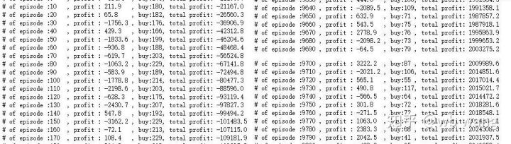
if n_epi%10==0:
print("# of episode :{:<5}, profit : {:<8.1f}, buy :{:<3}, sell :{:<3}, total profit: {:<20.1f}".format(n_epi, profit, buy_action, sell_action, total_profit))
7. Training results and analysis
After a long wait:

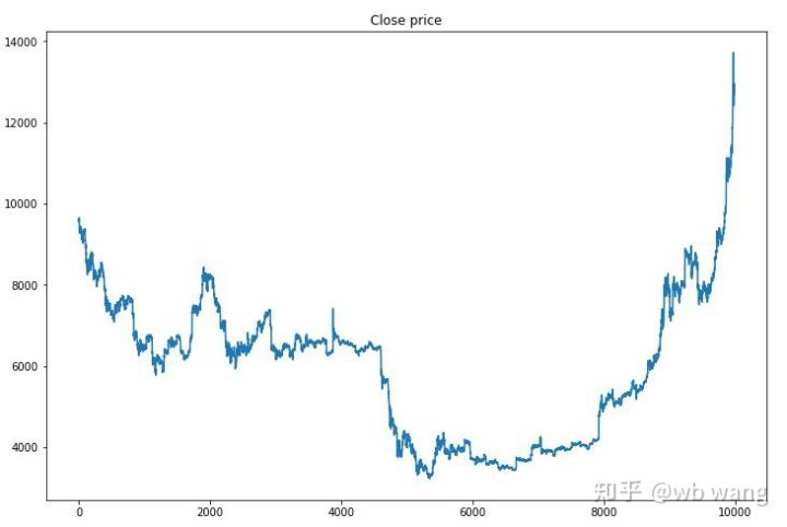
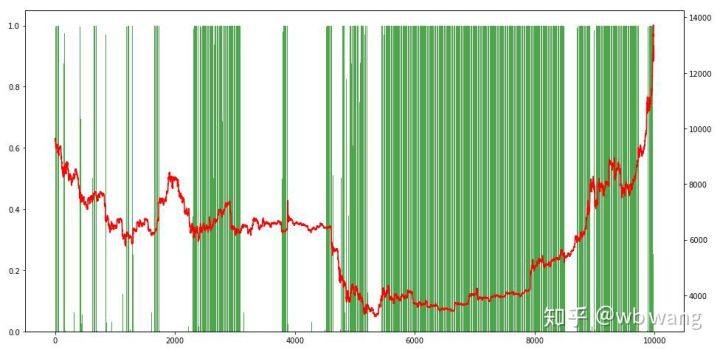
First of all, take a look at the market of training data. In general, the first half is a long-time decline, and the second half is a strong rebound.
There are many buying operations in the early stage of training, and there is basically no profitable round. By the middle of the training, the buying operation has gradually decreased, and the probability of profit is also increasing, but there is still a great chance of loss.
Smooth the profit of each round, and the result is as follows:
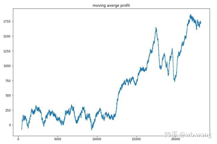
The strategy quickly got rid of the situation that the early return was negative, but the fluctuation was large. The return did not grow rapidly until after 10,000 rounds. In general, the model training was very difficult.
After the final training, let the model run all the data again to see how it performs. During the period, record the total market value of the account, the number of Bitcoins held, the proportion of Bitcoin value, and the total returns.
First is the total market value, and the total returns are similar to it, they will not be posted:
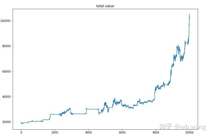
The total market value increased slowly in the early bear market, and kept up with the increase in the later bull market, but there were still periodic losses.
Finally, take a look at the proportion of positions. The left axis of the chart is the proportion of positions, and the right axis is the market. It can be preliminarily judged that the model is overfitting. The frequency of positions is low in the early bear market, and high at the bottom of the market. It can also be seen that the model has not learned to hold long-term positions and always sells quickly.
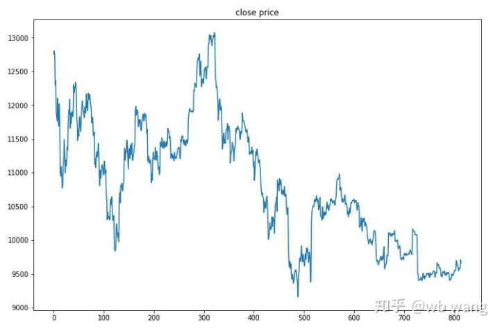
8. Test data analysis
The one-hour market of Bitcoin from June 27, 2019 till now was obtained from the test data. It can be seen from the chart that the price has dropped from $13,000 to more than $9,000, which is a great test for the model.
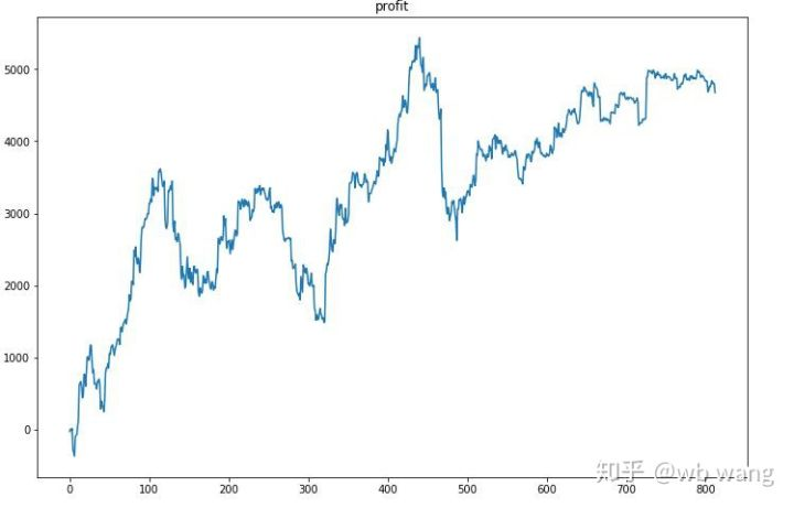
First of all, the final relative return performed so-so, but there was no loss.
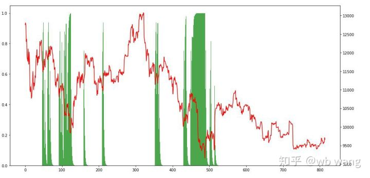
Looking at the position situation, we can guess that the model tends to buy after a sharp fall and sell after a rebound. The market of Bitcoin has fluctuated little in the recent period, and the model has been in a short position.
9. Summary
In this paper, a Bitcoin automatic trading robot is trained with the help of PPO, a deep intensive learning method, and some conclusions are obtained. Due to the limited time, there are still some aspects to be improved in the model. Welcome the discussion. The biggest lesson is that for data standardization method, don't use scaling and other methods, otherwise the model will quickly remember the relationship between price and market, and fall into overfitting. The standardized change rate is the relative data, which makes it difficult for the model to remember the relationship with the market, and is forced to find the relationship between the change rate and the increase and decrease.
Introduction to previous articles:
A high-frequency strategy I disclosed that was once very profitable: https://www.fmz.com/bbs-topic/9886.
- 1