Bitcoin price prediction in real time using the LSTM framework

Warning: This case is for study and research purposes only and does not constitute an investment proposal.

Bitcoin price data is based on time series, so Bitcoin price predictions are mostly done using the LSTM model.

Long-term short-term memory (LSTM) is a deep learning model specifically for time-series data (or data with a time/space/structure sequence, such as movies, sentences, etc.) that is an ideal model for predicting the price direction of cryptocurrencies.

This article mainly focuses on data matching using LSTM to predict the future price of Bitcoin.

Import libraries to use

import pandas as pd
import numpy as np

from sklearn.preprocessing import MinMaxScaler, LabelEncoder
from keras.models import Sequential
from keras.layers import LSTM, Dense, Dropout

from matplotlib import pyplot as plt
%matplotlib inline

Analysis of data

Loading of data

Read daily trading data for BTC

data = pd.read_csv(filepath_or_buffer="btc_data_day")

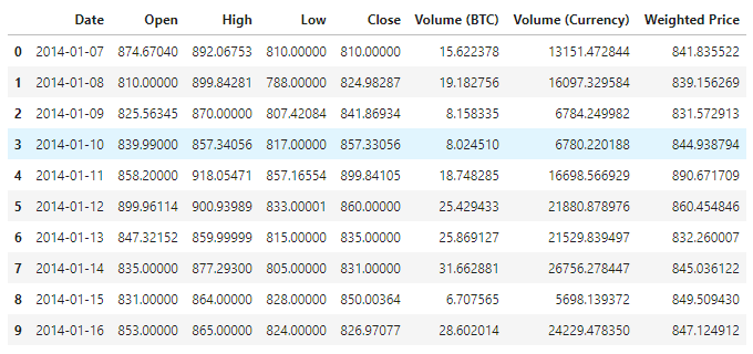
The data is available in a total of 1380 data items, consisting of the columns Date, Open, High, Low, Close, Volume (BTC), Volume (Currency) and Weighted Price. Except for the Date column, all other data columns are float64 data types.

data.info()

Check out the top 10 lines of data.

data.head(10)

Visualization of data

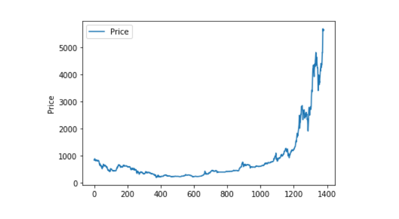
Using matplotlib, we plot the Weighted Price to see the distribution and trend of the data. In the graph, we find a section of data 0 that we need to confirm if there are any anomalies in the data.

plt.plot(data['Weighted Price'], label='Price')
plt.ylabel('Price')
plt.legend()
plt.show()

Unusual data processing

So let's see if the data contains nan data, and we can see that our data doesn't have nan data.

data.isnull().sum()

Date                 0
Open                 0
High                 0
Low                  0
Close                0
Volume (BTC)         0
Volume (Currency)    0
Weighted Price       0
dtype: int64

So if you look at the 0 data again, you can see that our data has a 0 value, and we need to process the 0 value.

(data == 0).astype(int).any()

Date                 False
Open                  True
High                  True
Low                   True
Close                 True
Volume (BTC)          True
Volume (Currency)     True
Weighted Price        True
dtype: bool

data['Weighted Price'].replace(0, np.nan, inplace=True)
data['Weighted Price'].fillna(method='ffill', inplace=True)
data['Open'].replace(0, np.nan, inplace=True)
data['Open'].fillna(method='ffill', inplace=True)
data['High'].replace(0, np.nan, inplace=True)
data['High'].fillna(method='ffill', inplace=True)
data['Low'].replace(0, np.nan, inplace=True)
data['Low'].fillna(method='ffill', inplace=True)
data['Close'].replace(0, np.nan, inplace=True)
data['Close'].fillna(method='ffill', inplace=True)
data['Volume (BTC)'].replace(0, np.nan, inplace=True)
data['Volume (BTC)'].fillna(method='ffill', inplace=True)
data['Volume (Currency)'].replace(0, np.nan, inplace=True)
data['Volume (Currency)'].fillna(method='ffill', inplace=True)

(data == 0).astype(int).any()

Date                 False
Open                 False
High                 False
Low                  False
Close                False
Volume (BTC)         False
Volume (Currency)    False
Weighted Price       False
dtype: bool

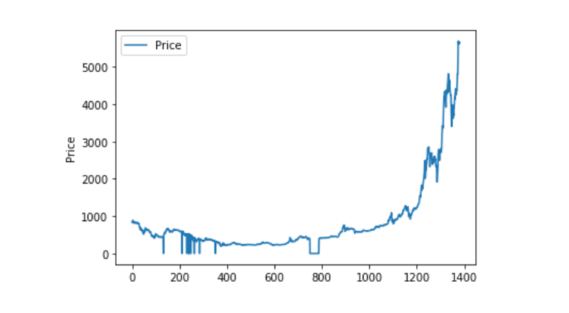
And then look at the distribution of the data and the trend, and the curve is very continuous at this point.

plt.plot(data['Weighted Price'], label='Price')
plt.ylabel('Price')
plt.legend()
plt.show()

Separation of training and test datasets

Unify the data to 0-1.

data_set = data.drop('Date', axis=1).values
data_set = data_set.astype('float32')
mms = MinMaxScaler(feature_range=(0, 1))
data_set = mms.fit_transform(data_set)

Divide the test and training datasets by 2:8.

ratio = 0.8
train_size = int(len(data_set) * ratio)
test_size = len(data_set) - train_size
train, test = data_set[0:train_size,:], data_set[train_size:len(data_set),:]

Create training and test datasets, and use one day as a window to create our training and test datasets.

def create_dataset(data):
    window = 1
    label_index = 6
    x, y = [], []
    for i in range(len(data) - window):
        x.append(data[i:(i + window), :])
        y.append(data[i + window, label_index])
    return np.array(x), np.array(y)

train_x, train_y = create_dataset(train)
test_x, test_y = create_dataset(test)

Defining and training models

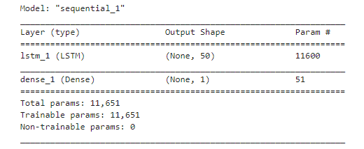
This time we used a simple model, which is structured as 1. LSTM2. Dense.

Input shapes have the input dimension of batch size, time steps, features. The time steps value is the time window interval at which the data is entered, where we use 1 day as the time window, and our data is day data, so our time steps are 1 here.

Long short-term memory (LSTM) is a special type of RNN that is primarily used to solve gradient disappearance and gradient explosion problems during long-series training.

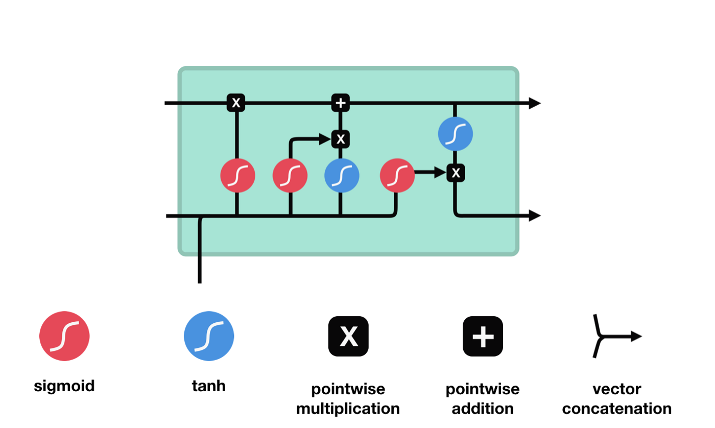
From the network structure diagram of the LSTM, it can be seen that the LSTM is actually a small model that contains 3 sigmoid activation functions, 2 tanh activation functions, 3 multiplication and 1 addition.

The state of cells

The state of the cell is the core of the LSTM, he is the black line at the top of the diagram above, and below this black line are some of the gates, which we will introduce later. The state of the cell will be updated according to the results of each gate.

The LSTM network removes or adds information about the state of the cell through a structure called a gate. The gate can selectively decide which information to let through. The gate is a combination of a sigmoid layer and a point multiplication operation.

The Forgotten Door

The first step of the LSTM is to decide what information the cell state needs to discard. This part of the operation is handled by a sigmoid unit called the forgetting gate.

We can see that the forgetting gate produces a vector between 0 and 1 by looking at the $h_{l-1}$ and $x_{t}$ messages, where the 0 to 1 value in the vector indicates how much information is retained or discarded in the cell state $C_{t-1}$. 0 indicates not retained, and 1 indicates retained.

The mathematical expression is $f_{t}=\sigma\left(W_{f} \cdot\left[h_{t-1}, x_{t}\right]+b_{f}\right) $

The entrance

The next step is to decide what new information to add to the cell state, which is done by opening the input gate.

We see that the information from $h_{l-1}$ and $x_{t}$ is again put into a forgetting gate (sigmoid) and input gate (tanh). Because the output of the forgetting gate is a value of 0-1, therefore, if the output of the forgetting gate is 0, the result after the input of the gate $C_{i}$ will not be added to the current cell state, if it is 1, it will all be added to the cell state, so the function of the forgetting gate here is to selectively add the result of the input gate to the cell state.

The mathematical formula is: $C_{t}=f_{t} * C_{t-1} + i_{t} * \tilde{C}_{t}$

The exit door

After updating the cell state, it is necessary to determine which state characteristics of the output cell are based on the sum of $h_{l-1}$ and $x_{t}$ inputs, where the input is obtained by passing through a sigmoid layer called the output gate, and then passing through the tanh layer to obtain a vector with a value between -1 and 1, which is multiplied by the input gate to obtain the output of the final RNN unit.

def create_model():
    model = Sequential()
    model.add(LSTM(50, input_shape=(train_x.shape[1], train_x.shape[2])))
    model.add(Dense(1))
    model.compile(loss='mae', optimizer='adam')
    model.summary()
    return model

model = create_model()

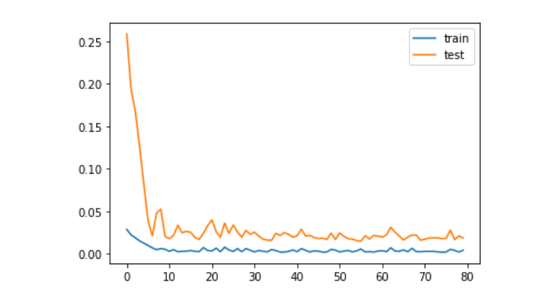
history = model.fit(train_x, train_y, epochs=80, batch_size=64, validation_data=(test_x, test_y), verbose=1, shuffle=False)

plt.plot(history.history['loss'], label='train')
plt.plot(history.history['val_loss'], label='test')
plt.legend()
plt.show()

train_x, train_y = create_dataset(train)
test_x, test_y = create_dataset(test)

Forecast

predict = model.predict(test_x)
plt.plot(predict, label='predict')
plt.plot(test_y, label='ground true')
plt.legend()
plt.show()

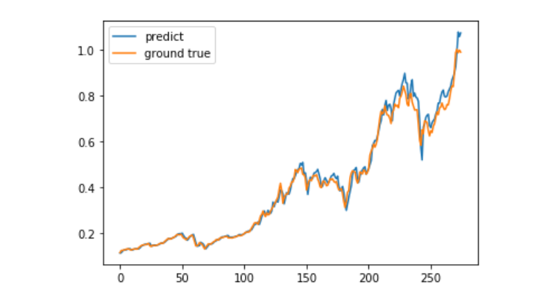
Currently, it is very difficult to use machine learning to predict the long-term price movement of Bitcoin, and this article can only be used as a case study. The case will then be launched with a demo image of the Matrix Cloud, which can be directly experienced by interested users.