An intraday trading strategy using the mean value return between SPY and IWM

In this article, we will write an intraday trading strategy. It will use the classic trading concept of the equity return trading pair. In this example, we will use two open-end exchange-traded funds (ETFs), SPY and IWM, which trade on the NYSE and attempt to represent the US stock market indices, the S&P 500 and the Russell 2000 respectively.

This strategy creates a profit differential by doing more than one ETF and doing nothing with another ETF. The multi-space ratio can be defined in many ways, such as using statistical synchronization time series methods. In this scenario, we will calculate the hedge ratio between SPY and IWM by rolling linear regression. This will allow us to create a profit differential between SPY and IWM, which is standardized as a z-score.

The basic premise of the strategy is that SPY and IWM both represent roughly the same market situation, that is, the stock price performance of a group of large and small U.S. companies. The premise is that if the price of the accepted parity of the parity of the parity of the parity of the parity of the parity of the parity of the parity of the parity of the parity of the parity of the parity of the parity of the parity of the parity of the parity of the parity of the parity of the parity of the parity of the parity of the parity of the parity of the parity of the parity of the parity of the parity of the parity of the parity of the parity of the parity of the parity of the parity of the parity of the parity of the parity of the parity of the parity of the parity of the parity of the parity of the parity of the parity of the parity of the parity of the parity of the parity of the parity of the parity of the parity of

The strategy

The strategy is implemented in the following steps:

Data - 1 minute k-string graphs obtained from SPY and IWM from April 2007 to February 2014 respectively.

Processing - aligning the data correctly and deleting k strings that are missing from each other.

Difference - The hedge ratio between the two ETFs is calculated using a rolling linear regression. Defined as the regression coefficient β using a regression window that moves the 1 k-line forward and recalculates the regression coefficient. Thus, the hedge ratio βi, the bi-root K-line is used to recall the k-line by computing the crossing point from bi-1-k to bi-1, which is used to recall the k-line.

Z-Score - The value of the standard deviation is calculated in the usual way. This means subtracting the mean value of the standard deviation from the sample and subtracting the standard deviation from the sample. The reason for doing this is to make the threshold parameter easier to understand, since the Z-Score is a dimensionless quantity.

Trading - when the negative z-score falls below the predetermined (or post-optimized) threshold, a do more signal is generated, while a do nothing signal is generated; when the absolute value of the z-score drops below the additional threshold, a placement signal is generated. For this strategy, I (somewhat randomly) chose z-score = 2 as the opening threshold, and z-score = 1 as the placement threshold.

Perhaps the best way to get a deeper understanding of the policy is to actually implement it. The following section details the full Python code used to implement this even-valued return policy (single file). I have added a detailed code commentary to help you better understand.

Implementation of Python

As with all Python/pandas tutorials, it must be set up according to the Python environment described in this tutorial. Once setup is complete, the first task is to import the necessary Python library. This is necessary for using matplotlib and pandas.

The specific library versions I use are as follows:

Python - 2.7.3 NumPy - 1.8.0 pandas - 0.12.0 matplotlib - 1.1.0

Let's go ahead and import these libraries:

# mr_spy_iwm.py

import matplotlib.pyplot as plt
import numpy as np
import os, os.path
import pandas as pd

The following function create_pairs_dataframe imports two intrinsic k-strings of CSV files containing two symbols. In our example, this would be SPY and IWM. It then creates a separate array of data pairs, which will use the indexes of the two original files. Their timelines can vary due to missed transactions and errors.

# mr_spy_iwm.py
def create_pairs_dataframe(datadir, symbols):
    """Creates a pandas DataFrame containing the closing price
    of a pair of symbols based on CSV files containing a datetime
    stamp and OHLCV data."""
 
    # Open the individual CSV files and read into pandas DataFrames
    print "Importing CSV data..."
    sym1 = pd.io.parsers.read_csv(os.path.join(datadir, '%s.csv' % symbols[0]),
                                  header=0, index_col=0, 
                                  names=['datetime','open','high','low','close','volume','na'])
    sym2 = pd.io.parsers.read_csv(os.path.join(datadir, '%s.csv' % symbols[1]),
                                  header=0, index_col=0, 
                                  names=['datetime','open','high','low','close','volume','na'])
 
    # Create a pandas DataFrame with the close prices of each symbol
    # correctly aligned and dropping missing entries
    print "Constructing dual matrix for %s and %s..." % symbols    
    pairs = pd.DataFrame(index=sym1.index)
    pairs['%s_close' % symbols[0].lower()] = sym1['close']
    pairs['%s_close' % symbols[1].lower()] = sym2['close']
    pairs = pairs.dropna()
    return pairs

The next step is to roll linear regression between SPY and IWM. In this scenario, IWM is the predictor (x) and SPY is the response (y). I set a default regression window of 100 k-strings. As mentioned above, this is a parameter of the policy. In order for the policy to be considered robust, we would ideally like to see a return report display convex function states (x) or other performance metric performance in the regression period.

After calculating the rolling beta coefficient in the linear regression model of SPY-IWM, add it to the DataFrame pairs and remove the blank lines. This builds the first set of K-lines, which is equal to a retrograde length trimming measure. Then, we create two ETFs with dividends, units of SPY and units of -βi of IWM. Obviously, this is not realistic because we are using a small amount of IWM, which is not possible in the actual implementation.

Finally, we create a z-score of the spread, calculated by subtracting the mean of the spread and using the standard deviation of the standard deviation. Note that there is a rather subtle bias here. I intentionally left it in the code because I wanted to emphasize how easy it is to make such mistakes in research.

# mr_spy_iwm.py
 
def calculate_spread_zscore(pairs, symbols, lookback=100):
    """Creates a hedge ratio between the two symbols by calculating
    a rolling linear regression with a defined lookback period. This
    is then used to create a z-score of the 'spread' between the two
    symbols based on a linear combination of the two."""
     
    # Use the pandas Ordinary Least Squares method to fit a rolling
    # linear regression between the two closing price time series
    print "Fitting the rolling Linear Regression..."
    model = pd.ols(y=pairs['%s_close' % symbols[0].lower()], 
                   x=pairs['%s_close' % symbols[1].lower()],
                   window=lookback)
 
    # Construct the hedge ratio and eliminate the first 
    # lookback-length empty/NaN period
    pairs['hedge_ratio'] = model.beta['x']
    pairs = pairs.dropna()
 
    # Create the spread and then a z-score of the spread
    print "Creating the spread/zscore columns..."
    pairs['spread'] = pairs['spy_close'] - pairs['hedge_ratio']*pairs['iwm_close']
    pairs['zscore'] = (pairs['spread'] - np.mean(pairs['spread']))/np.std(pairs['spread'])
    return pairs

In create_long_short_market_signals, create trading signals. These are calculated by the value of the z-score exceeding the threshold. When the absolute value of the z-score is less than or equal to another (smaller) threshold, a breakeven signal is given.

In order to achieve this, it is necessary to establish a trading strategy for each k-string to be open-ended or flat-ended. Long_market and short_market are the two defined variables used to track both multi-head and empty-head positions. Unfortunately, it is easier to program in an iterative manner compared to the vector method and therefore is slow to compute. Although a 1-minute k-string chart requires about 700,000 data points per CSV file, it is still relatively fast to compute on my old desktop!

To iterate a pandas DataFrame (which is undoubtedly an uncommon operation), it is necessary to use the iterrows method, which provides an iterative generator:

# mr_spy_iwm.py
 
def create_long_short_market_signals(pairs, symbols, 
                                     z_entry_threshold=2.0, 
                                     z_exit_threshold=1.0):
    """Create the entry/exit signals based on the exceeding of 
    z_enter_threshold for entering a position and falling below
    z_exit_threshold for exiting a position."""
 
    # Calculate when to be long, short and when to exit
    pairs['longs'] = (pairs['zscore'] <= -z_entry_threshold)*1.0
    pairs['shorts'] = (pairs['zscore'] >= z_entry_threshold)*1.0
    pairs['exits'] = (np.abs(pairs['zscore']) <= z_exit_threshold)*1.0
 
    # These signals are needed because we need to propagate a
    # position forward, i.e. we need to stay long if the zscore
    # threshold is less than z_entry_threshold by still greater
    # than z_exit_threshold, and vice versa for shorts.
    pairs['long_market'] = 0.0
    pairs['short_market'] = 0.0
 
    # These variables track whether to be long or short while
    # iterating through the bars
    long_market = 0
    short_market = 0
 
    # Calculates when to actually be "in" the market, i.e. to have a
    # long or short position, as well as when not to be.
    # Since this is using iterrows to loop over a dataframe, it will
    # be significantly less efficient than a vectorised operation,
    # i.e. slow!
    print "Calculating when to be in the market (long and short)..."
    for i, b in enumerate(pairs.iterrows()):
        # Calculate longs
        if b[1]['longs'] == 1.0:
            long_market = 1            
        # Calculate shorts
        if b[1]['shorts'] == 1.0:
            short_market = 1
        # Calculate exists
        if b[1]['exits'] == 1.0:
            long_market = 0
            short_market = 0
        # This directly assigns a 1 or 0 to the long_market/short_market
        # columns, such that the strategy knows when to actually stay in!
        pairs.ix[i]['long_market'] = long_market
        pairs.ix[i]['short_market'] = short_market
    return pairs

At this stage, we updated the pairs to include actual multiple, blank signals, which enabled us to determine if we needed to open a position. Now we need to create a portfolio to track the market value of the position. The first task is to create a position column that combines multiple signals and blank signals. This will contain a row of elements from ((1, 0, -1), where 1 represents multiple positions, 0 represents no positions (should be flat), and -1 represents blank positions.

Once the market value of the ETF has been created, we combine them to produce the total market value at the end of each k-line. Then we convert it to the return value via the pct_change method of the object. The subsequent lines of code clear the incorrect entries (NaN and inf elements) and finally calculate the complete interest curve.

# mr_spy_iwm.py
 
def create_portfolio_returns(pairs, symbols):
    """Creates a portfolio pandas DataFrame which keeps track of
    the account equity and ultimately generates an equity curve.
    This can be used to generate drawdown and risk/reward ratios."""
     
    # Convenience variables for symbols
    sym1 = symbols[0].lower()
    sym2 = symbols[1].lower()
 
    # Construct the portfolio object with positions information
    # Note that minuses to keep track of shorts!
    print "Constructing a portfolio..."
    portfolio = pd.DataFrame(index=pairs.index)
    portfolio['positions'] = pairs['long_market'] - pairs['short_market']
    portfolio[sym1] = -1.0 * pairs['%s_close' % sym1] * portfolio['positions']
    portfolio[sym2] = pairs['%s_close' % sym2] * portfolio['positions']
    portfolio['total'] = portfolio[sym1] + portfolio[sym2]
 
    # Construct a percentage returns stream and eliminate all 
    # of the NaN and -inf/+inf cells
    print "Constructing the equity curve..."
    portfolio['returns'] = portfolio['total'].pct_change()
    portfolio['returns'].fillna(0.0, inplace=True)
    portfolio['returns'].replace([np.inf, -np.inf], 0.0, inplace=True)
    portfolio['returns'].replace(-1.0, 0.0, inplace=True)
 
    # Calculate the full equity curve
    portfolio['returns'] = (portfolio['returns'] + 1.0).cumprod()
    return portfolio

The main function combines them. The CSV file is located in the datadir path. Be sure to modify the following code to point to your specific directory.

In order to determine the sensitivity of the strategy to lookback cycles, it is necessary to calculate a series of lookback performance indicators. I chose the final total return percentage of the portfolio as a performance indicator and lookback range[50,200], incremented by 10. You can see in the code below that the previous function is contained in the for loop within this range, with the other thresholds remaining unchanged. The final task is to create a line graph of lookbacks versus returns using matplotlib:

# mr_spy_iwm.py
 
if __name__ == "__main__":
    datadir = '/your/path/to/data/'  # Change this to reflect your data path!
    symbols = ('SPY', 'IWM')
 
    lookbacks = range(50, 210, 10)
    returns = []
 
    # Adjust lookback period from 50 to 200 in increments
    # of 10 in order to produce sensitivities
    for lb in lookbacks: 
        print "Calculating lookback=%s..." % lb
        pairs = create_pairs_dataframe(datadir, symbols)
        pairs = calculate_spread_zscore(pairs, symbols, lookback=lb)
        pairs = create_long_short_market_signals(pairs, symbols, 
                                                z_entry_threshold=2.0, 
                                                z_exit_threshold=1.0)
 
        portfolio = create_portfolio_returns(pairs, symbols)
        returns.append(portfolio.ix[-1]['returns'])
 
    print "Plot the lookback-performance scatterchart..."
    plt.plot(lookbacks, returns, '-o')
    plt.show()

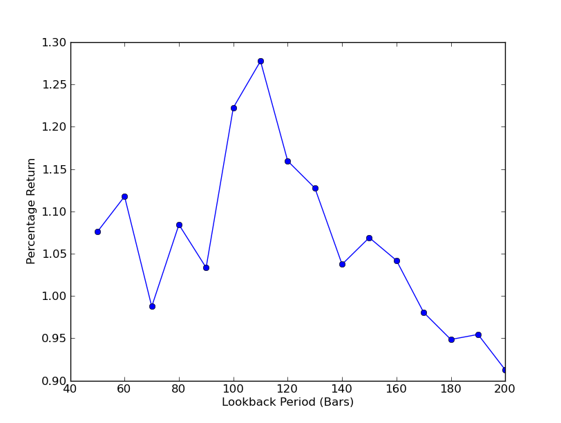
Now you can see a graph of lookbacks and returns. Note that lookbacks have a maximum value of a diagonal globally, equal to 110 k lines. If we see that lookbacks are unrelated to returns, this is because:

SPY-IWM linear regression hedge versus lookback period sensitivity analysis

Without an upward sloping profit curve, any retrospective article is incomplete! Therefore, if you want to plot a curve of cumulative profit returns and time, you can use the following code. It will plot the final portfolio generated from the lookback parameter study. It is therefore necessary to select a lookback based on the chart you want to visualize.

# mr_spy_iwm.py
 
    # This is still within the main function
    print "Plotting the performance charts..."
    fig = plt.figure()
    fig.patch.set_facecolor('white')
 
    ax1 = fig.add_subplot(211,  ylabel='%s growth (%%)' % symbols[0])
    (pairs['%s_close' % symbols[0].lower()].pct_change()+1.0).cumprod().plot(ax=ax1, color='r', lw=2.)
 
    ax2 = fig.add_subplot(212, ylabel='Portfolio value growth (%%)')
    portfolio['returns'].plot(ax=ax2, lw=2.)
 
    fig.show()

Lookback period for the following rights-benefit curve chart is 100 days:

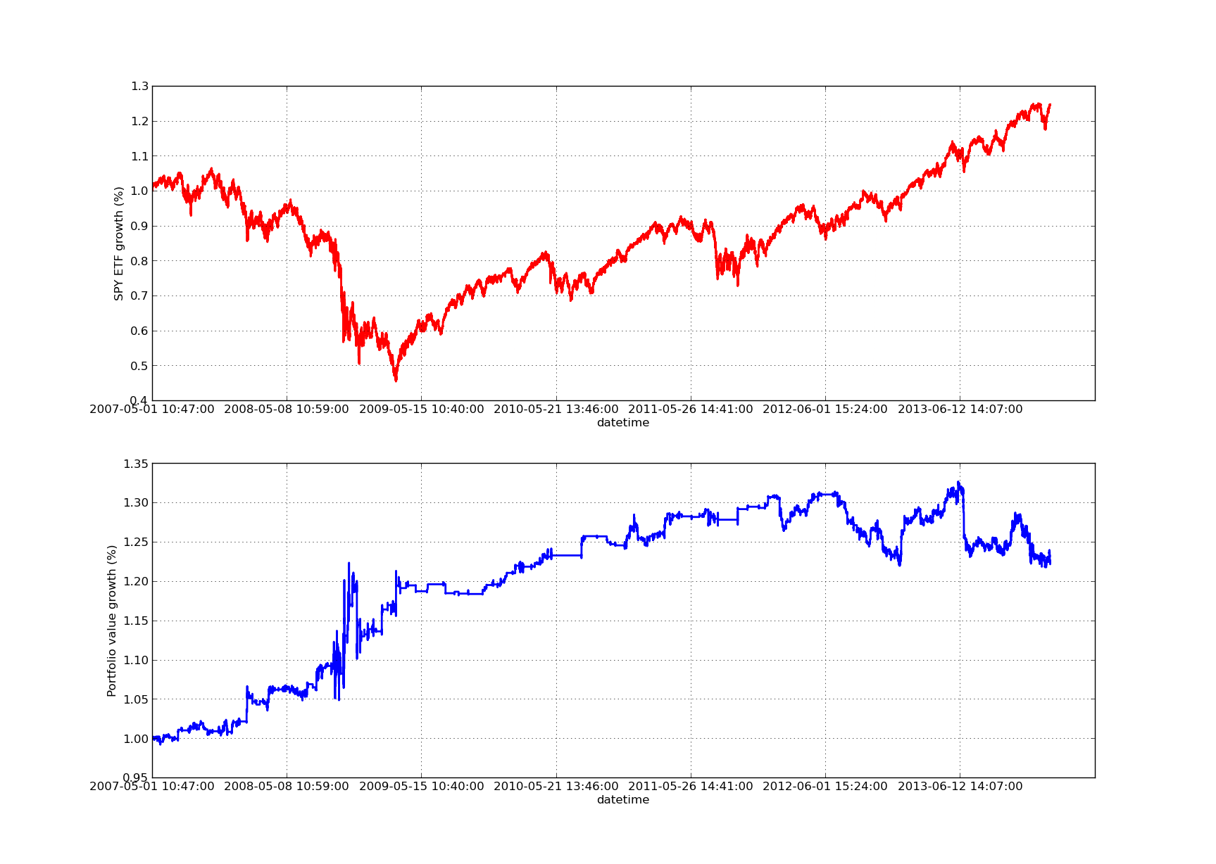
SPY-IWM linear regression hedge versus lookback period sensitivity analysis

Please note that the 2009 SPY contracted significantly during the financial crisis. The strategy was also in turmoil at this stage. Please also note that last year's performance deteriorated due to the strongly trendy nature of the SPY during this period, reflecting the S&P 500 index.

Note that we still need to consider the forward bias bias bias when calculating the z-score. Furthermore, all of these calculations were done in the absence of transaction costs. Once these factors are taken into account, this strategy is sure to perform poorly. The fees and slippage points are currently uncertain.

In a later article, we will create a more sophisticated event-driven backtester that will take these factors into account, giving us more confidence in the capital curve and performance indicators.