Pairing trades are a good example of developing a trading strategy based on mathematical analysis. In this article, we will demonstrate how to use data to create and automate pairing trading strategies.

Basic Principles

假设你有一对投资标的X和Y具有一些潜在的关联，例如两家公司生产相同的产品，如百事可乐和可口可乐。你希望这两者的价格比率或基差（也称为差价）随时间的变化而保持不变。然而，由于临时供需变化，如一个投资标的的大买/卖订单，对其中一家公司的重要新闻的反应等，这两对之间的价差可能会不时出现分歧。在这种情况下，一只投资标的向上移动而另一只投资标的相对于彼此向下移动。如果你希望这种分歧随着时间的推移恢复正常，你就可以发现交易机会(或套利机会)。此种套利机会在数字货币市场或者国内商品期货市场比比皆是,比如BTC与避险资产的关系;期货中豆粕,豆油与大豆品种之间的关系.

When there is a temporary price difference, the trade will sell the upper-performing investment and buy the lower-performing investment. You can be sure that the difference between the two investments will eventually result in either a fall in the upper-performing investment or a rebound in the lower-performing investment or both. Your trade will make money in all of these similar scenarios.

Thus, paired trading is a market-neutral trading strategy that enables traders to profit from almost any market condition: uptrend, downtrend, or horizontal placement.

Explanation of the concept: two hypothetical investment indicators

• Inventors are building our research environment on a quantified platform.

First of all, in order for the work to proceed smoothly, we need to build our research environment, which we use in this article as an inventor quantification platform.FMZ.COMThe purpose of the project is to build a research environment, mainly for the convenient and fast API interfaces and well-wrapped Docker systems that can be used later on.

In the official name of the inventor's quantification platform, this Docker system is called the host system.

For more information on how to deploy hosts and bots, please refer to my previous post:https://www.fmz.com/bbs-topic/4140

Readers who want to buy their own cloud server deployment host can refer to this article:https://www.fmz.com/bbs-topic/2848

After successfully deploying a good cloud service and host system, next we'll install Python's biggest temple to date: Anaconda.

The easiest way to implement all the relevant programming environments (dependencies, version management, etc.) is to use Anaconda. It is a packed Python data science ecosystem and dependency library manager.

For instructions on how to install Anaconda, please see the official guide to Anaconda:https://www.anaconda.com/distribution/

本文还将用到numpy和pandas这两个目前在Python科学计算方面十分流行且重要的库.

These basics can also be referenced in my previous article on how to set up the Anaconda environment and the numpy and pandas libraries.https://www.fmz.com/digest-topic/4169

Next, let's use the code to implement a "two hypothesis investment criterion".

import numpy as np
import pandas as pd

import statsmodels
from statsmodels.tsa.stattools import coint
# just set the seed for the random number generator
np.random.seed(107)

import matplotlib.pyplot as plt

Yes, we're also going to use the chart library in the very famous Python library, matplotlib.

Let's generate an X of a hypothetical investment indicator and simulate its daily return by using a normal distribution. Then we perform cumulative addition to get the daily X value.

# Generate daily returns
Xreturns = np.random.normal(0, 1, 100) 
# sum them and shift all the prices up
X = pd.Series(np.cumsum(
    Xreturns), name='X') 
    + 50
X.plot(figsize=(15,7))
plt.show()

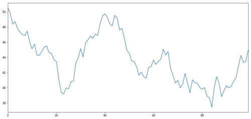
X of the investment indicator, simulating its daily return by normal distribution

Now the Y we generate is strongly correlated with X, so the price of Y should be very similar to the change in X. We model this by taking X, moving it up and adding some random noise extracted from the normal distribution.

noise = np.random.normal(0, 1, 100)
Y = X + 5 + noise
Y.name = 'Y'
pd.concat([X, Y], axis=1).plot(figsize=(15,7))
plt.show()

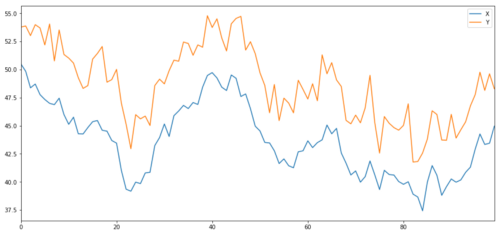
X and Y of the co-ordinated investment indicator

Coordinated

协整非常类似于相关性，意味着两个数据系列之间的比率将在平均值附近变化.Y和X这两个系列遵循以下内容：

Y = ⍺ X + e

where r is the constant ratio and e is the noise.

For transaction pairs between two time sequences, the ratio must converge over time to the expected value of the homogeneity, i.e. they should be co-integral. The time sequence we constructed above is co-integral. We will now plot the ratio between the two so that we can see what it looks like.

(Y/X).plot(figsize=(15,7)) 
plt.axhline((Y/X).mean(), color='red', linestyle='--') 
plt.xlabel('Time')
plt.legend(['Price Ratio', 'Mean'])
plt.show()

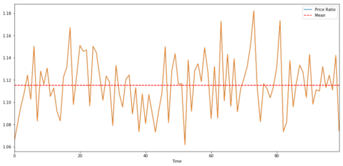
Ratio and average between the prices of two converging investment indicators

Collaborative testing

There is a convenient test method, which is to use statsmodels.tsa.stattools. We should see a very low p-value because we have artificially created two sets of data that are as close together as possible.

# compute the p-value of the cointegration test
# will inform us as to whether the ratio between the 2 timeseries is stationary
# around its mean
score, pvalue, _ = coint(X,Y)
print pvalue

The result is: 1.81864477307e-17

Note: Relevance and coherence

Related and coherent, although similar in theory, are not the same thing. Let's look at examples of data series that are related but not coherent, and vice versa. First, let's check the correlation of the series we just generated.

X.corr(Y)

The result is: 0.951.

As we would expect, this is very high. But what about two related but disjoint series? A simple example is two divergent data series.

ret1 = np.random.normal(1, 1, 100)
ret2 = np.random.normal(2, 1, 100)

s1 = pd.Series( np.cumsum(ret1), name='X')
s2 = pd.Series( np.cumsum(ret2), name='Y')

pd.concat([s1, s2], axis=1 ).plot(figsize=(15,7))
plt.show()
print 'Correlation: ' + str(X_diverging.corr(Y_diverging))
score, pvalue, _ = coint(X_diverging,Y_diverging)
print 'Cointegration test p-value: ' + str(pvalue)

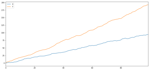
Two related series (not integrated)

Related coefficients: 0.998 The p-value of the co-integration test: 0.258

Simple examples of non-correlation co-integration are the normal distribution sequence and the square wave.

Y2 = pd.Series(np.random.normal(0, 1, 800), name='Y2') + 20
Y3 = Y2.copy()

Y3[0:100] = 30
Y3[100:200] = 10
Y3[200:300] = 30
Y3[300:400] = 10
Y3[400:500] = 30
Y3[500:600] = 10
Y3[600:700] = 30
Y3[700:800] = 10
Y2.plot(figsize=(15,7))
Y3.plot()
plt.ylim([0, 40])
plt.show()
# correlation is nearly zero
print 'Correlation: ' + str(Y2.corr(Y3))
score, pvalue, _ = coint(Y2,Y3)
print 'Cointegration test p-value: ' + str(pvalue)

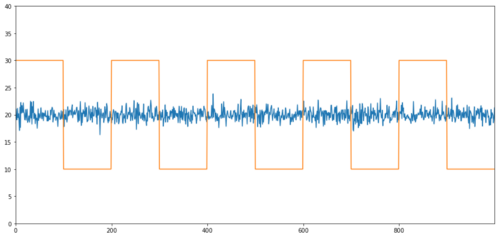
This is the first time I've seen this. The p-value of the co-integration test: 0.0

The correlation is very low, but the p-value shows perfect synergy!

How do you do the pairing?

Because two concurrent time series (e.g. X and Y above) are aligned and diverging from each other, there are sometimes high and low marginal differences. We do a paired trade by buying one asset and selling another. Thus, if the two assets fall or rise together, we neither make nor lose money, i.e. we are neutral in the market.

Going back to the above Y = X + e in X and Y, so that the ratio ((Y / X) moves around its mean value curve, we make money by the ratio of the mean return. To do this, we pay attention to the case when X and Y are far apart, i.e. the threshold is too high or too low:

• Do more ratios: This is when the ratio is very small and we expect it to get bigger. In the example above, we open a position by doing more Y and doing empty X.

• Blank ratio: This is when the ratio is very high and we expect it to change hours. In the example above, we open the position by blank Y and doing more X.

Note that we always have a hedged position hedge: if the trade's buy-loss value, the empty position will make money, and vice versa, so we are immune to the overall market movement.

If the X and Y of the trade moves relative to each other, we make money or lose money.

Use data to search for similar transactional indicators

The best way to do this is to start with the trade indicator you suspect might be a synergy and perform a statistical test.Multiple comparison biasThe victims of the massacre.

Multiple comparison biasRefers to the increased chance of incorrectly generating important p-values when running multiple tests, because we need to run multiple tests. If we run 100 tests on random data, we should see 5 p-values less than 0.05. If you were to compare n transaction indicators to make an integer, you would perform n − 1 / 2 comparisons, and you would see many incorrect p-values, which would increase as your test sample increased. To avoid this, select a small number of pairs of transactions for which you have reason to believe that they may be compatible, and then test them separately. This would greatly reduce the number of false p-values.Multiple comparison bias。

So let's try to find some indices that show synergies. Let's take the example of a basket of large US tech stocks in the S&P 500 that operate in similar segments of the market and have synergies.

Returns all pairs of the co-integral check fraction matrix, p-value matrix, and p-value less than 0.05.This method is prone to multiple comparison biases, so they actually need to perform a secondary verification.In this article, for the sake of our explanation, we choose to ignore this in the example.

def find_cointegrated_pairs(data):
    n = data.shape[1]
    score_matrix = np.zeros((n, n))
    pvalue_matrix = np.ones((n, n))
    keys = data.keys()
    pairs = []
    for i in range(n):
        for j in range(i+1, n):
            S1 = data[keys[i]]
            S2 = data[keys[j]]
            result = coint(S1, S2)
            score = result[0]
            pvalue = result[1]
            score_matrix[i, j] = score
            pvalue_matrix[i, j] = pvalue
            if pvalue < 0.02:
                pairs.append((keys[i], keys[j]))
    return score_matrix, pvalue_matrix, pairs

Note: We have included in the data the market benchmark (SPX) - the market drives the movement of many trading indices, and often you may find two seemingly synchronized trading indices; but in reality they do not synchronize with each other, but with the market. This is called a mixed variable.

from backtester.dataSource.yahoo_data_source import YahooStockDataSource
from datetime import datetime
startDateStr = '2007/12/01'
endDateStr = '2017/12/01'
cachedFolderName = 'yahooData/'
dataSetId = 'testPairsTrading'
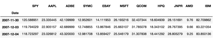
instrumentIds = ['SPY','AAPL','ADBE','SYMC','EBAY','MSFT','QCOM',
                 'HPQ','JNPR','AMD','IBM']
ds = YahooStockDataSource(cachedFolderName=cachedFolderName,
                            dataSetId=dataSetId,
                            instrumentIds=instrumentIds,
                            startDateStr=startDateStr,
                            endDateStr=endDateStr,
                            event='history')
data = ds.getBookDataByFeature()['Adj Close']
data.head(3)

Now let's try to use our method to find a symmetrical transaction pairing.

# Heatmap to show the p-values of the cointegration test
# between each pair of stocks
scores, pvalues, pairs = find_cointegrated_pairs(data)
import seaborn
m = [0,0.2,0.4,0.6,0.8,1]
seaborn.heatmap(pvalues, xticklabels=instrumentIds, 
                yticklabels=instrumentIds, cmap=’RdYlGn_r’, 
                mask = (pvalues >= 0.98))
plt.show()
print pairs

[('ADBE', 'MSFT')]

It looks like ADBE and MSFT are working together. Let's take a look at the price to make sure it really makes sense.

S1 = data['ADBE']
S2 = data['MSFT']
score, pvalue, _ = coint(S1, S2)
print(pvalue)
ratios = S1 / S2
ratios.plot()
plt.axhline(ratios.mean())
plt.legend([' Ratio'])
plt.show()

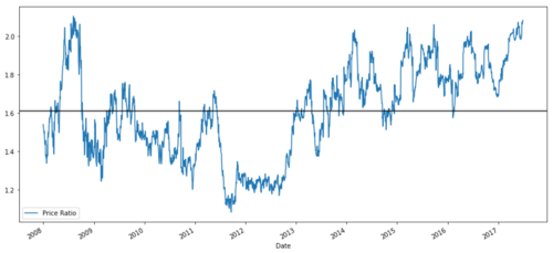
Graph of price ratio between MSFT and ADBE 2008 - 2017

This ratio does look like a stable mean. Absolute ratios are not very useful statistically. It is more helpful to standardize our signal by treating it as a z-score. Z-score is defined as:

Z Score (Value) = (Value — Mean) / Standard Deviation

Warning

In fact, we usually try to make some extensions to the data, but on the assumption that the data are normal distributions. However, many financial data are not normal distributions, so we have to be very careful not to simply assume normality or any specific distribution when generating statistics. The true distribution of ratios can have a fat tail effect, and those that tend to extremes can confuse our models and cause huge losses.

def zscore(series):
    return (series - series.mean()) / np.std(series)

zscore(ratios).plot()
plt.axhline(zscore(ratios).mean())
plt.axhline(1.0, color=’red’)
plt.axhline(-1.0, color=’green’)
plt.show()

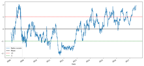
Z-price ratio between MSFT and ADBE between 2008 and 2017

It is now easier to observe ratios moving near the mean, but sometimes it is easy to see large differences with the mean, which we can exploit.

Now that we've discussed the basics of pairing trading strategies and identified a commonly integrated trading indicator based on historical prices, let's try developing a trading signal. First, let's review the steps of developing trading signals using data technology:

• Collect reliable data and clean up data

• Create functions from data to identify trading signals/logic

• Functions can be moving averages or price data, correlations or ratios of more complex signals - combine these to create new features

• These functions are used to generate trading signals, i.e. which signals are buy, sell or hold

Fortunately, we have inventors to quantify the platform.fmz.comThis is a huge boon for strategy developers, who can put their energy and time into designing and extending the functionality of the strategy logic.

In the inventor quantification platform, there are interfaces packaged for all kinds of mainstream exchanges, all we have to do is call these APIs, and the rest of the underlying implementation logic, which has already been polished by a professional team.

For the sake of completeness of the logic and explanation of the principles, we will present these underlying logics in the form of a bulldozer, but in practical operation, you can directly call the inventor's quantized API interface to complete the above four aspects.

Let's start with:

Step 1: Set your problems

Here, we try to create a signal that tells us whether the ratio is buying or selling at the next moment, which is our prediction variable Y:

Y = Ratio is buy (1) or sell (-1)

Y(t)= Sign(Ratio(t+1) — Ratio(t))

Note that we don't need to predict the price of the actual trade mark, or even the actual value of the ratio (although we can), we just need to predict the direction of the ratio next.

Step 2: Collect reliable and accurate data

The inventor quantification is your friend! You just specify the trade mark to be traded and the data source to be used, and it extracts the data you need and cleans it up for dividend and trade mark decomposition.

We have the following data from the last 10 trading days (about 2500 data points) using Yahoo Finance: opening price, closing price, highest price, lowest price and trading volume.

Step three: Split the data

Don't forget this very important step to test model accuracy. We are using the following data for training/validation/testing breakdowns

• Training 7 years ~ 70%

• Test ~ 3 years 30%

ratios = data['ADBE'] / data['MSFT']
print(len(ratios))
train = ratios[:1762]
test = ratios[1762:]

Ideally, we should also make a verification set, but we won't do that for now.

Step four: Characterization

What can be the related function? We want to predict the direction of the change in the ratio. We have seen that our two trade indicators are convergent, so the ratio tends to shift and return to the mean. It seems that our feature should be some measure of the mean of the ratio, the difference between the current value and the mean that can produce our trading signal.

We use the following functions:

• 60 day moving average: measurement of rolling averages

• 5-day moving average ratio: Measurement of the current value of the average

• Standard deviation of 60 days

• The z-score: ((5d MA - 60d MA) / 60d SD

ratios_mavg5 = train.rolling(window=5,
                               center=False).mean()
ratios_mavg60 = train.rolling(window=60,
                               center=False).mean()
std_60 = train.rolling(window=60,
                        center=False).std()
zscore_60_5 = (ratios_mavg5 - ratios_mavg60)/std_60
plt.figure(figsize=(15,7))
plt.plot(train.index, train.values)
plt.plot(ratios_mavg5.index, ratios_mavg5.values)
plt.plot(ratios_mavg60.index, ratios_mavg60.values)
plt.legend(['Ratio','5d Ratio MA', '60d Ratio MA'])
plt.ylabel('Ratio')
plt.show()

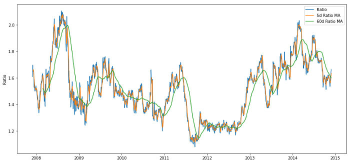
Price ratio of 60d and 5d MA

plt.figure(figsize=(15,7))
zscore_60_5.plot()
plt.axhline(0, color='black')
plt.axhline(1.0, color='red', linestyle='--')
plt.axhline(-1.0, color='green', linestyle='--')
plt.legend(['Rolling Ratio z-Score', 'Mean', '+1', '-1'])
plt.show()

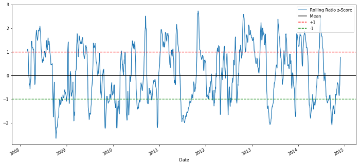
60-5 Z score price ratio

The z-score of the rolling mean does bring out the mean regression nature of the ratio!

Step five: Model selection

Let's start with a very simple model. Look at the z-score graph, and we can see that as long as the z-score is too high or too low, it will return. Let's use +1/-1 as our threshold to define too high and too low, and then we can use the following model to generate a trading signal:

• When z is less than -1.0, the ratio is buy (-1), because we expect z to return to 0, so the ratio increases.

• When z is greater than 1.0, the ratio is sold (−1) because we expect z to return to 0, so the ratio decreases.

Step six: train, verify and optimize

And finally, let's look at the actual effect of our model on the actual data.

# Plot the ratios and buy and sell signals from z score
plt.figure(figsize=(15,7))
train[60:].plot()
buy = train.copy()
sell = train.copy()
buy[zscore_60_5>-1] = 0
sell[zscore_60_5<1] = 0
buy[60:].plot(color=’g’, linestyle=’None’, marker=’^’)
sell[60:].plot(color=’r’, linestyle=’None’, marker=’^’)
x1,x2,y1,y2 = plt.axis()
plt.axis((x1,x2,ratios.min(),ratios.max()))
plt.legend([‘Ratio’, ‘Buy Signal’, ‘Sell Signal’])
plt.show()

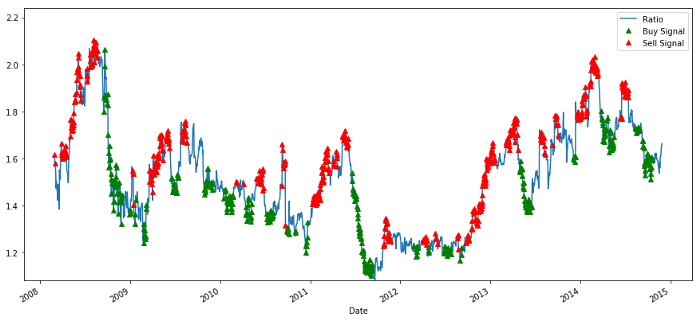
Buy and sell price ratio signals

This signal seems reasonable, we seem to sell the ratio when it's high or increasing and buy back when it's low (green) and decreasing. What does this mean for the actual trading indicator we're trading?

# Plot the prices and buy and sell signals from z score
plt.figure(figsize=(18,9))
S1 = data['ADBE'].iloc[:1762]
S2 = data['MSFT'].iloc[:1762]
S1[60:].plot(color='b')
S2[60:].plot(color='c')
buyR = 0*S1.copy()
sellR = 0*S1.copy()
# When buying the ratio, buy S1 and sell S2
buyR[buy!=0] = S1[buy!=0]
sellR[buy!=0] = S2[buy!=0]
# When selling the ratio, sell S1 and buy S2 
buyR[sell!=0] = S2[sell!=0]
sellR[sell!=0] = S1[sell!=0]
buyR[60:].plot(color='g', linestyle='None', marker='^')
sellR[60:].plot(color='r', linestyle='None', marker='^')
x1,x2,y1,y2 = plt.axis()
plt.axis((x1,x2,min(S1.min(),S2.min()),max(S1.max(),S2.max())))
plt.legend(['ADBE','MSFT', 'Buy Signal', 'Sell Signal'])
plt.show()

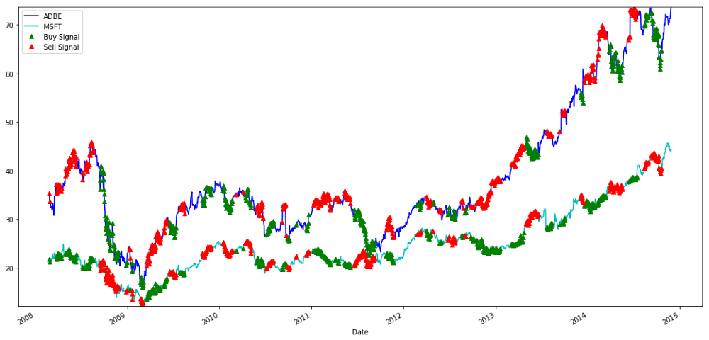
Signals for buying and selling MSFT and ADBE stocks

Note how we sometimes make money on "short legs", sometimes on "long legs", and sometimes both.

We are satisfied with the signal of the training data. Let's see what kind of profit this signal can generate. When the ratio is low, we can make a simple backmeter, buy 1 ratio (buy 1 ADBE stock and sell ratio x MSFT stock) and sell 1 ratio when it is high (sell 1 ADBE stock and buy ratio x MSFT stock) and calculate the PnL of these ratios.

# Trade using a simple strategy
def trade(S1, S2, window1, window2):
    
    # If window length is 0, algorithm doesn't make sense, so exit
    if (window1 == 0) or (window2 == 0):
        return 0
    
    # Compute rolling mean and rolling standard deviation
    ratios = S1/S2
    ma1 = ratios.rolling(window=window1,
                               center=False).mean()
    ma2 = ratios.rolling(window=window2,
                               center=False).mean()
    std = ratios.rolling(window=window2,
                        center=False).std()
    zscore = (ma1 - ma2)/std
    
    # Simulate trading
    # Start with no money and no positions
    money = 0
    countS1 = 0
    countS2 = 0
    for i in range(len(ratios)):
        # Sell short if the z-score is > 1
        if zscore[i] > 1:
            money += S1[i] - S2[i] * ratios[i]
            countS1 -= 1
            countS2 += ratios[i]
            print('Selling Ratio %s %s %s %s'%(money, ratios[i], countS1,countS2))
        # Buy long if the z-score is < 1
        elif zscore[i] < -1:
            money -= S1[i] - S2[i] * ratios[i]
            countS1 += 1
            countS2 -= ratios[i]
            print('Buying Ratio %s %s %s %s'%(money,ratios[i], countS1,countS2))
        # Clear positions if the z-score between -.5 and .5
        elif abs(zscore[i]) < 0.75:
            money += S1[i] * countS1 + S2[i] * countS2
            countS1 = 0
            countS2 = 0
            print('Exit pos %s %s %s %s'%(money,ratios[i], countS1,countS2))
            
            
    return money
trade(data['ADBE'].iloc[:1763], data['MSFT'].iloc[:1763], 60, 5)

The result is: 1783.375.

So this strategy seems to be profitable! Now, we can further optimize by changing the moving average time window, by changing the buy/sell thresholds of the peak position, etc., and check the performance improvement of the verification data.

We can also try more complex models, such as Logistic Regression, SVM, etc., to make 1/-1 predictions.

Now, let's move this model forward, and this brings us to

Step 7: Reassess the test data

The inventor's quantification platform uses a high-performance QPS/TPS backtesting engine to recreate historical environments in real time, eliminating common quantification backtesting pitfalls and detecting shortcomings in strategies in a timely manner to better assist real-time investing.

This article explains the principle, or chooses to show the underlying logic, in practical application, or recommends that readers use the inventor quantification platform, in addition to saving time, it is important to improve the error tolerance.

The retest is very simple, and we can use the function above to look at the PnL of the test data.

trade(data[‘ADBE’].iloc[1762:], data[‘MSFT’].iloc[1762:], 60, 5)

The result was: 5262.868.

The model worked well! It became our first simple pairing-to-transaction model.

Avoid over-fitting

Before concluding the discussion, I would like to specifically discuss over-fitting. Over-fitting is the most dangerous trap in trading strategies. Over-fitting algorithms can perform very well in retrospective but fail on new invisible data - which means that it doesn't really reveal any trends in the data and doesn't have any real predictive power.

In our model, we use rolling parameter predictions and hope to optimize the length of the time window by them. We may decide to simply iterate through all possibilities, a reasonable time window length, and choose the length of time based on how well our model performs. Below we write a simple loop to score the length of the time window based on the training data and find the optimal loop.

# Find the window length 0-254 
# that gives the highest returns using this strategy
length_scores = [trade(data['ADBE'].iloc[:1762], 
                data['MSFT'].iloc[:1762], l, 5) 
                for l in range(255)]
best_length = np.argmax(length_scores)
print ('Best window length:', best_length)

('Best window length:', 40)

Now we check the model's performance on the test data, and we find that the length of this time window is far from optimal! This is because our original selection obviously over-matched the sample data.

# Find the returns for test data
# using what we think is the best window length
length_scores2 = [trade(data['ADBE'].iloc[1762:], 
                  data['MSFT'].iloc[1762:],l,5) 
                  for l in range(255)]
print (best_length, 'day window:', length_scores2[best_length])
# Find the best window length based on this dataset, 
# and the returns using this window length
best_length2 = np.argmax(length_scores2)
print (best_length2, 'day window:', length_scores2[best_length2])

(40, 'day window:', 1252233.1395)
(15, 'day window:', 1449116.4522)

Obviously the data that fits our sample doesn't always produce good results in the future. Just for testing, let's plot the length fraction calculated from the two datasets.

plt.figure(figsize=(15,7))
plt.plot(length_scores)
plt.plot(length_scores2)
plt.xlabel('Window length')
plt.ylabel('Score')
plt.legend(['Training', 'Test'])
plt.show()

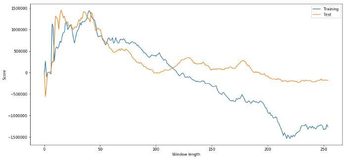
We can see that anything between 20-50 is a good option for the time window.

To avoid over-fitting, we can use the nature of economic reasoning or algorithms to select the length of a time window. We can also use a Kallman filter, which does not require us to specify the length; this method will be introduced later in another article.

The next step

In this article, we offer some simple introductory methods to demonstrate the process of developing a trading strategy. In practice, more complex statistics should be used, and the following options can be considered:

• The Hurst Index

• Half-life of the mean value regression inferred from the Ornstein-Uhlenbeck process

• The Kalman filter

Related

More