Factor model of digital currency

[TOC]

Factor model framework

The research report on the multi-factor model of the stock market can be said to be sweat-filled, with rich theories and practices. The digital currency market is sufficient to satisfy for factor research regardless of the number of coins, total market value, transaction volume, derivatives market, etc. This article is mainly addressed to beginners of quantitative strategies, does not involve complex mathematical principles and statistical analysis, will use the currency futures market as a data source, construct a simple framework for factor research, and make it convenient to evaluate factor indicators.

A factor can be thought of as an indicator, written as an expression, a constantly changing factor that reflects future earnings information, usually a factor that represents an investment logic.

For example: the closing price close factor, the assumption behind which is that the stock price can predict future returns, the higher the stock price, the higher the future returns (or possibly the lower), the fact that the portfolio is actually an investment model/strategy of buying high-priced stocks on a regular basis. Generally speaking, those factors that can generate sustained excess returns are often referred to as alpha. For example, market value factors, momentum factors, etc. have been proven by the academic and investment community to be once effective factors.

Both the stock market and the digital currency market are a complex system, with no factors that can fully predict future returns, but still have a certain predictability. Effective alpha (investment model) and gradually fail as more funds are put in. But this process will lead to other patterns in the market, giving rise to new alphas. The market value factor was once a very effective strategy in the A stock market, simply buying 10 stocks with the lowest market value, adjusting once a day, and will get a return of more than 400 times the reassessment, far exceeding the profit margin from the decade of 2007. But the big alpha 2017 stock market reflects the failure of the small market factor, the value factor instead became popular.

The factors that are sought are the foundation of strategy building, and a better strategy can be constructed by combining multiple unrelated effective factors.

import requests
from datetime import date,datetime
import time
import pandas as pd
import numpy as np
import matplotlib.pyplot as plt
import requests, zipfile, io
%matplotlib inline

Source of the data

The hourly K-line data from the beginning of 2022 to the present date, so far, has more than 150 currencies. As mentioned earlier, the factor model is a currency model that is aimed at all currencies, rather than a particular currency. The K-line data contains data on high and low opening prices, transactions, transactions, active purchases, etc., which of course are not the source of all factors, such as the US stock index, interest rate increases, profitability expectations, data on the chain, social media heat, etc. Cold-door data sources may also find effective alphas, but basic price data is also quite sufficient.

## 当前交易对
Info = requests.get('https://fapi.binance.com/fapi/v1/exchangeInfo')
symbols = [s['symbol'] for s in Info.json()['symbols']]
symbols = list(filter(lambda x: x[-4:] == 'USDT', [s.split('_')[0] for s in symbols]))
print(symbols)

Out:

['BTCUSDT', 'ETHUSDT', 'BCHUSDT', 'XRPUSDT', 'EOSUSDT', 'LTCUSDT', 'TRXUSDT', 'ETCUSDT', 'LINKUSDT',
'XLMUSDT', 'ADAUSDT', 'XMRUSDT', 'DASHUSDT', 'ZECUSDT', 'XTZUSDT', 'BNBUSDT', 'ATOMUSDT', 'ONTUSDT',
'IOTAUSDT', 'BATUSDT', 'VETUSDT', 'NEOUSDT', 'QTUMUSDT', 'IOSTUSDT', 'THETAUSDT', 'ALGOUSDT', 'ZILUSDT',
'KNCUSDT', 'ZRXUSDT', 'COMPUSDT', 'OMGUSDT', 'DOGEUSDT', 'SXPUSDT', 'KAVAUSDT', 'BANDUSDT', 'RLCUSDT',
'WAVESUSDT', 'MKRUSDT', 'SNXUSDT', 'DOTUSDT', 'DEFIUSDT', 'YFIUSDT', 'BALUSDT', 'CRVUSDT', 'TRBUSDT',
'RUNEUSDT', 'SUSHIUSDT', 'SRMUSDT', 'EGLDUSDT', 'SOLUSDT', 'ICXUSDT', 'STORJUSDT', 'BLZUSDT', 'UNIUSDT',
'AVAXUSDT', 'FTMUSDT', 'HNTUSDT', 'ENJUSDT', 'FLMUSDT', 'TOMOUSDT', 'RENUSDT', 'KSMUSDT', 'NEARUSDT',
'AAVEUSDT', 'FILUSDT', 'RSRUSDT', 'LRCUSDT', 'MATICUSDT', 'OCEANUSDT', 'CVCUSDT', 'BELUSDT', 'CTKUSDT',
'AXSUSDT', 'ALPHAUSDT', 'ZENUSDT', 'SKLUSDT', 'GRTUSDT', '1INCHUSDT', 'CHZUSDT', 'SANDUSDT', 'ANKRUSDT',
'BTSUSDT', 'LITUSDT', 'UNFIUSDT', 'REEFUSDT', 'RVNUSDT', 'SFPUSDT', 'XEMUSDT', 'BTCSTUSDT', 'COTIUSDT',
'CHRUSDT', 'MANAUSDT', 'ALICEUSDT', 'HBARUSDT', 'ONEUSDT', 'LINAUSDT', 'STMXUSDT', 'DENTUSDT', 'CELRUSDT',
'HOTUSDT', 'MTLUSDT', 'OGNUSDT', 'NKNUSDT', 'SCUSDT', 'DGBUSDT', '1000SHIBUSDT', 'ICPUSDT', 'BAKEUSDT',
'GTCUSDT', 'BTCDOMUSDT', 'TLMUSDT', 'IOTXUSDT', 'AUDIOUSDT', 'RAYUSDT', 'C98USDT', 'MASKUSDT', 'ATAUSDT',
'DYDXUSDT', '1000XECUSDT', 'GALAUSDT', 'CELOUSDT', 'ARUSDT', 'KLAYUSDT', 'ARPAUSDT', 'CTSIUSDT', 'LPTUSDT',
'ENSUSDT', 'PEOPLEUSDT', 'ANTUSDT', 'ROSEUSDT', 'DUSKUSDT', 'FLOWUSDT', 'IMXUSDT', 'API3USDT', 'GMTUSDT',
'APEUSDT', 'BNXUSDT', 'WOOUSDT', 'FTTUSDT', 'JASMYUSDT', 'DARUSDT', 'GALUSDT', 'OPUSDT', 'BTCUSDT',
'ETHUSDT', 'INJUSDT', 'STGUSDT', 'FOOTBALLUSDT', 'SPELLUSDT', '1000LUNCUSDT', 'LUNA2USDT', 'LDOUSDT',
'CVXUSDT']

---

print(len(symbols))

Out:

153

---

#获取任意周期K线的函数
def GetKlines(symbol='BTCUSDT',start='2020-8-10',end='2021-8-10',period='1h',base='fapi',v = 'v1'):
    Klines = []
    start_time = int(time.mktime(datetime.strptime(start, "%Y-%m-%d").timetuple()))*1000 + 8*60*60*1000
    end_time =  min(int(time.mktime(datetime.strptime(end, "%Y-%m-%d").timetuple()))*1000 + 8*60*60*1000,time.time()*1000)
    intervel_map = {'m':60*1000,'h':60*60*1000,'d':24*60*60*1000}
    while start_time < end_time:
        mid_time = start_time+1000*int(period[:-1])*intervel_map[period[-1]]
        url = 'https://'+base+'.binance.com/'+base+'/'+v+'/klines?symbol=%s&interval=%s&startTime=%s&endTime=%s&limit=1000'%(symbol,period,start_time,mid_time)
        res = requests.get(url)
        res_list = res.json()
        if type(res_list) == list and len(res_list) > 0:
            start_time = res_list[-1][0]+int(period[:-1])*intervel_map[period[-1]]
            Klines += res_list
        if type(res_list) == list and len(res_list) == 0:
            start_time = start_time+1000*int(period[:-1])*intervel_map[period[-1]]
        if mid_time >= end_time:
            break
    df = pd.DataFrame(Klines,columns=['time','open','high','low','close','amount','end_time','volume','count','buy_amount','buy_volume','null']).astype('float')
    df.index = pd.to_datetime(df.time,unit='ms')
    return df

start_date = '2022-1-1'
end_date = '2022-09-14'
period = '1h'
df_dict = {}
for symbol in symbols:
    df_s = GetKlines(symbol=symbol,start=start_date,end=end_date,period=period,base='fapi',v='v1')
    if not df_s.empty:
        df_dict[symbol] = df_s

symbols = list(df_dict.keys())
print(df_s.columns)

Out:

Index(['time', 'open', 'high', 'low', 'close', 'amount', 'end_time', 'volume',
       'count', 'buy_amount', 'buy_volume', 'null'],
      dtype='object')

---

Initially, we extract the data we are interested in from the K-line data: closing price, opening price, volume of transactions, number of transactions, percentage of active purchases, and then process the necessary factors based on these data.

df_close = pd.DataFrame(index=pd.date_range(start=start_date, end=end_date, freq=period),columns=df_dict.keys())
df_open = pd.DataFrame(index=pd.date_range(start=start_date, end=end_date, freq=period),columns=df_dict.keys())
df_volume = pd.DataFrame(index=pd.date_range(start=start_date, end=end_date, freq=period),columns=df_dict.keys())
df_buy_ratio = pd.DataFrame(index=pd.date_range(start=start_date, end=end_date, freq=period),columns=df_dict.keys())
df_count = pd.DataFrame(index=pd.date_range(start=start_date, end=end_date, freq=period),columns=df_dict.keys())
for symbol in df_dict.keys():
    df_s = df_dict[symbol]
    df_close[symbol] = df_s.close
    df_open[symbol] = df_s.open
    df_volume[symbol] = df_s.volume
    df_count[symbol] = df_s['count']
    df_buy_ratio[symbol] = df_s.buy_amount/df_s.amount
df_close = df_close.dropna(how='all')
df_open = df_open.dropna(how='all')
df_volume = df_volume.dropna(how='all')
df_count = df_count.dropna(how='all')
df_buy_ratio = df_buy_ratio.dropna(how='all')

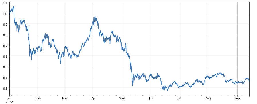
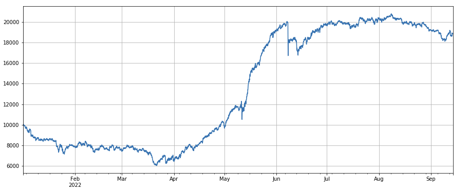
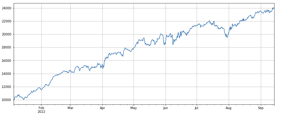
The overall performance of the market index, which has fallen by 60% since the beginning of the year, is somewhat dismal.

df_norm = df_close/df_close.fillna(method='bfill').iloc[0] #归一化
df_norm.mean(axis=1).plot(figsize=(15,6),grid=True);
#最终指数收益图

Determination of factor efficacy

• The Law of Regression In the following phase, the yield is used as a dependent variable, the factor to be tested as a self-variable, and the returned coefficient is the yield of the factor. After constructing the regression equation, the absolute mean of the coefficient t-value is generally referenced, the proportion of the series of absolute values of the coefficient t-value greater than 2, the annualized factor yield, the annualized factor yield fluctuation rate, the sharpness of the ratio of the factor gain, etc. parameters to see the effectiveness and volatility of the factor.

• Indicators such as IC, IR The so-called IC is the coefficient between the factor rank and the next period's yield, now also commonly used as the RANK_IC, which is the coefficient between the factor rank and the next period's stock yield. IR is generally the mean value of the IC series/standard deviation of the IC series.

• Layered regression This article will use this method, which is to divide the coins into N groups according to the order of the factors to be tested, to perform a reclassification, and to use a fixed period to perform the positioning operation. If the situation is ideal, the yield of the N group of coins will show better monotony, monotony increases or decreases, and the yield gap between each group is larger. Such a factor is reflected in a better differentiation. If the first group yields the highest, the last group yields the lowest, then the first combination is made and the last combination is made more empty, the final resulting yield, the reference indicator of the Sharpe ratio.

Practical retesting operations

The smaller the number of coins, the higher the return, but also the greater the amount of money allocated to each coin. If the first and last sets of 10 coins are multiplied by a factor, the ratio is 10%, and if the number of coins is multiplied by a factor, it is 20%; if the corresponding set of 50 coins is multiplied by a factor, it is 20%; if the corresponding set of 50 coins is multiplied by a factor, it is 20%.

The predictive power of the factors can usually be roughly assessed by the yield and Sharpe ratio of the final retest. It is also necessary to consider whether the factor expression is simple, insensitive to the size of the cluster, insensitive to the adjustment interval, insensitive to the initial time of retest, etc.

In terms of frequency, the stock market tends to cycle for 5 days, 10 days and a month, but for the digital currency market, such cycles are undoubtedly too long, and the market is monitored in real time, so it is not necessary to reset a specific cycle, so in real time we are real-time or short-term cyclical trading.

As for how to equalize, according to the traditional method, the next sort can be equalized without being in the group; but in the case of real-time trading, some currencies may be right on the dividing line, and there will be a situation of back and forth equalization. Therefore, this strategy uses the waiting group change, and when the position needs to be reversed, it is necessary to equalize again, such as when the first group is more, and when the currencies in the multi-state are divided into a third group, it is necessary to equalize again. If the fixed equilibrium cycle, such as every day or every 8 hours, it is also possible to use the non-group method of equalize.

#回测引擎
class Exchange:
    
    def __init__(self, trade_symbols, fee=0.0004, initial_balance=10000):
        self.initial_balance = initial_balance #初始的资产
        self.fee = fee
        self.trade_symbols = trade_symbols
        self.account = {'USDT':{'realised_profit':0, 'unrealised_profit':0, 'total':initial_balance, 'fee':0, 'leverage':0, 'hold':0}}
        for symbol in trade_symbols:
            self.account[symbol] = {'amount':0, 'hold_price':0, 'value':0, 'price':0, 'realised_profit':0,'unrealised_profit':0,'fee':0}
            
    def Trade(self, symbol, direction, price, amount):
        
        cover_amount = 0 if direction*self.account[symbol]['amount'] >=0 else min(abs(self.account[symbol]['amount']), amount)
        open_amount = amount - cover_amount
        self.account['USDT']['realised_profit'] -= price*amount*self.fee #扣除手续费
        self.account['USDT']['fee'] += price*amount*self.fee
        self.account[symbol]['fee'] += price*amount*self.fee

        if cover_amount > 0: #先平仓
            self.account['USDT']['realised_profit'] += -direction*(price - self.account[symbol]['hold_price'])*cover_amount  #利润
            self.account[symbol]['realised_profit'] += -direction*(price - self.account[symbol]['hold_price'])*cover_amount
            
            self.account[symbol]['amount'] -= -direction*cover_amount
            self.account[symbol]['hold_price'] = 0 if self.account[symbol]['amount'] == 0 else self.account[symbol]['hold_price']
            
        if open_amount > 0:
            total_cost = self.account[symbol]['hold_price']*direction*self.account[symbol]['amount'] + price*open_amount
            total_amount = direction*self.account[symbol]['amount']+open_amount
            
            self.account[symbol]['hold_price'] = total_cost/total_amount
            self.account[symbol]['amount'] += direction*open_amount
                    
    
    def Buy(self, symbol, price, amount):
        self.Trade(symbol, 1, price, amount)
        
    def Sell(self, symbol, price, amount):
        self.Trade(symbol, -1, price, amount)
        
    def Update(self, close_price): #对资产进行更新
        self.account['USDT']['unrealised_profit'] = 0
        self.account['USDT']['hold'] = 0
        for symbol in self.trade_symbols:
            if not np.isnan(close_price[symbol]):
                self.account[symbol]['unrealised_profit'] = (close_price[symbol] - self.account[symbol]['hold_price'])*self.account[symbol]['amount']
                self.account[symbol]['price'] = close_price[symbol]
                self.account[symbol]['value'] = abs(self.account[symbol]['amount'])*close_price[symbol]
                self.account['USDT']['hold'] += self.account[symbol]['value']
                self.account['USDT']['unrealised_profit'] += self.account[symbol]['unrealised_profit']
        self.account['USDT']['total'] = round(self.account['USDT']['realised_profit'] + self.initial_balance + self.account['USDT']['unrealised_profit'],6)
        self.account['USDT']['leverage'] = round(self.account['USDT']['hold']/self.account['USDT']['total'],3)

#测试因子的函数
def Test(factor, symbols, period=1, N=40, value=300):
    e = Exchange(symbols, fee=0.0002, initial_balance=10000)
    res_list = []
    index_list = []
    factor = factor.dropna(how='all')
    for idx, row in factor.iterrows():
        if idx.hour % period == 0:
            buy_symbols =  row.sort_values().dropna()[0:N].index
            sell_symbols = row.sort_values().dropna()[-N:].index
            prices = df_close.loc[idx,]
            index_list.append(idx)
            for symbol in symbols:
                if symbol in buy_symbols and e.account[symbol]['amount'] <= 0:
                    e.Buy(symbol,prices[symbol],value/prices[symbol]-e.account[symbol]['amount'])
                if symbol in sell_symbols and e.account[symbol]['amount'] >= 0:
                    e.Sell(symbol,prices[symbol], value/prices[symbol]+e.account[symbol]['amount'])
            e.Update(prices)
            res_list.append([e.account['USDT']['total'],e.account['USDT']['hold']])
    return pd.DataFrame(data=res_list, columns=['total','hold'],index = index_list)

Simple factor tests

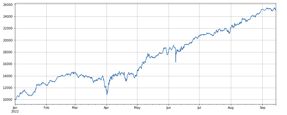
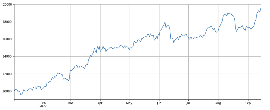
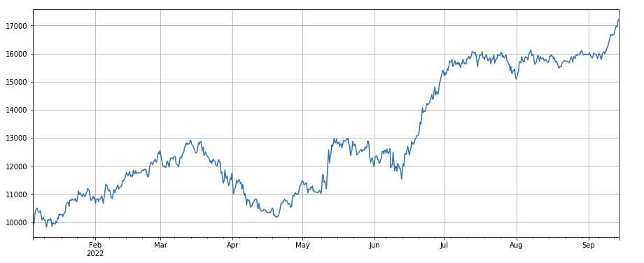
Trading factor: Currencies with low trading volume and high trading volume perform very well, which indicates that hot coins tend to fall.

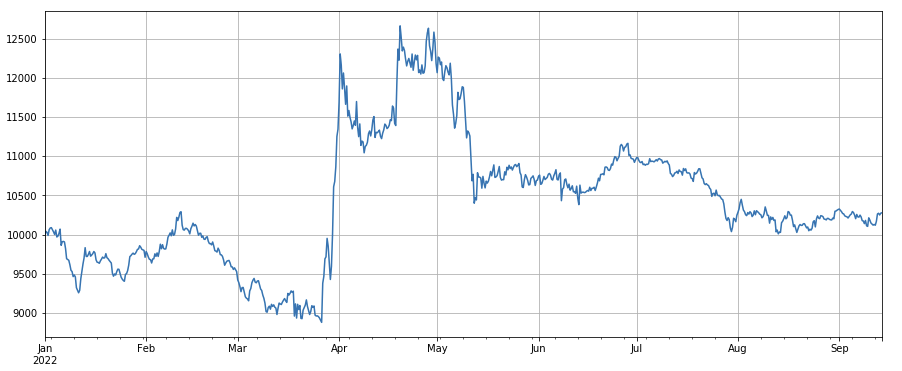
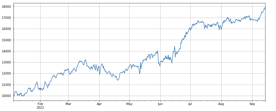
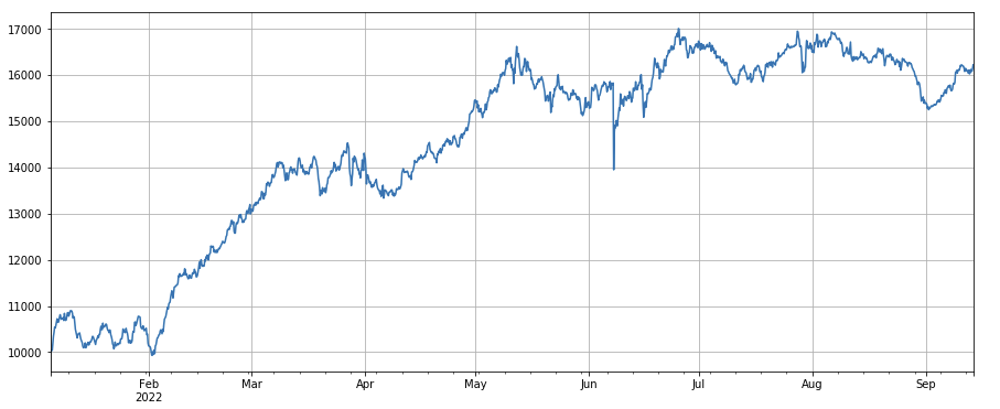
The transaction price factor: low-priced currencies, high-priced currencies, general effect.

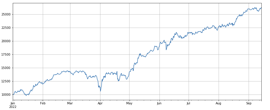
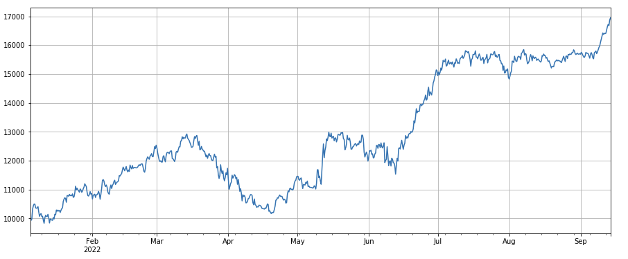
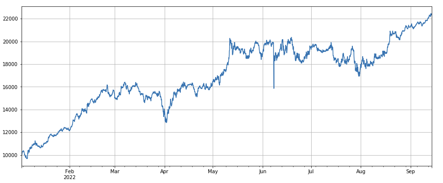
Transaction number factor: Performance and transaction number are very similar. It can be clearly noted that the correlation between the transaction number factor and the transaction number factor is very high, and in fact, the average correlation between their different currencies reaches 0.97, which indicates that the two factors are very close, and this factor needs to be taken into account when synthesizing a multifactor.

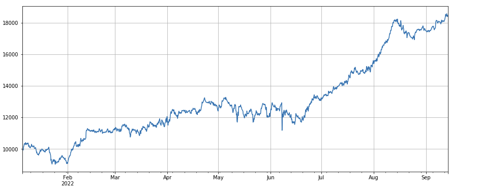
3h momentum factor: ((df_close - df_close.shift)) 3)) /df_close.shift ((3)); i.e. the factor's 3-hour increase, the retest results show that the 3-hour increase has a pronounced regression characteristic, i.e. the upward is then more likely to fall. The overall performance is good, but there is also a longer retracement and oscillation period.

24h momentum factor: 24h reset cycle results are good, the gain is close to 3h momentum and the retracement is smaller.

The change in the volume of the trade:df_volume.rolling ((24).mean)) /df_volume.rolling ((96).mean ((), i.e. the ratio of the volume of the trade in the last 1 day to the volume of the trade in the last 3 days, adjusted once every 8 hours. The retest performance is better, the retracement is also lower, which indicates that the trade is active and tends to fall.

The change in the number of transactions:df_count.rolling ((24).mean)) /df_count.rolling ((96).mean ((), i.e. the ratio of the number of transactions in the last 1 day to the number of transactions in the last 3 days, adjusted once every 8 hours. The retest performance was better, the retracement was also lower, which indicates that the number of transactions increased actively rather than tending to fall.

Factors of change in the value of single transactions: - ((df_volume.rolling(24).mean()/df_count.rolling(24).mean())/ ((df_volume.rolling(24).mean()/df_count.rolling(96).mean()) This is the ratio of the value of the most recent one-day transaction to the value of the most recent three-day transaction, every 8 hours. This factor is also highly correlated with the volume factor.

Active transaction ratio change factor:df_buy_ratio.rolling ((24).mean (() /df_buy_ratio.rolling ((96).mean (())), i.e. the ratio of active purchase volume to total transaction volume in the last 1 day to the ratio of transaction value in the last 3 days, once every 8 hours. This factor is still present, and the correlation with the transaction volume factor is not very large.

The volatility factor: (df_close/df_open).rolling (df_close/df_open).rolling (df_close/df_open).std (df_std))), which makes the multi-volatility of the currency small, has a certain effect.

Df_close.rolling ((96).corr ((df_volume), the last 4 days of closing prices have a correlation factor of the volume of transactions, the overall performance is good.

These are just a few of the factors that are based on the quantity-value basis. In fact, the combinations of factor formulas can be very complex and can have no obvious logic.https://github.com/STHSF/alpha101 。

#成交量
factor_volume = df_volume
factor_volume_res = Test(factor_volume, symbols, period=4)
factor_volume_res.total.plot(figsize=(15,6),grid=True);

#成交价
factor_close = df_close
factor_close_res = Test(factor_close, symbols, period=8)
factor_close_res.total.plot(figsize=(15,6),grid=True);

#成交笔数
factor_count = df_count
factor_count_res = Test(factor_count, symbols, period=8)
factor_count_res.total.plot(figsize=(15,6),grid=True);

print(df_count.corrwith(df_volume).mean())

0.9671246744996017

#3小时动量因子
factor_1 =  (df_close - df_close.shift(3))/df_close.shift(3)
factor_1_res = Test(factor_1,symbols,period=1)
factor_1_res.total.plot(figsize=(15,6),grid=True);

#24小时动量因子
factor_2 =  (df_close - df_close.shift(24))/df_close.shift(24)
factor_2_res = Test(factor_2,symbols,period=24)
tamenxuanfactor_2_res.total.plot(figsize=(15,6),grid=True);

#成交量因子
factor_3 = df_volume.rolling(24).mean()/df_volume.rolling(96).mean()
factor_3_res = Test(factor_3, symbols, period=8)
factor_3_res.total.plot(figsize=(15,6),grid=True);

#成交笔数因子
factor_4 = df_count.rolling(24).mean()/df_count.rolling(96).mean()
factor_4_res = Test(factor_4, symbols, period=8)
factor_4_res.total.plot(figsize=(15,6),grid=True);

#因子相关性
print(factor_4.corrwith(factor_3).mean())

0.9707239580854841

#单笔成交价值因子
factor_5 = -(df_volume.rolling(24).mean()/df_count.rolling(24).mean())/(df_volume.rolling(24).mean()/df_count.rolling(96).mean())
factor_5_res = Test(factor_5, symbols, period=8)
factor_5_res.total.plot(figsize=(15,6),grid=True);

print(factor_4.corrwith(factor_5).mean())

0.861206620552479

#主动成交比例因子
factor_6 = df_buy_ratio.rolling(24).mean()/df_buy_ratio.rolling(96).mean()
factor_6_res = Test(factor_6, symbols, period=4)
factor_6_res.total.plot(figsize=(15,6),grid=True);

print(factor_3.corrwith(factor_6).mean())

0.1534572192503726

#波动率因子
factor_7 = (df_close/df_open).rolling(24).std()
factor_7_res = Test(factor_7, symbols, period=2)
factor_7_res.total.plot(figsize=(15,6),grid=True);

#成交量和收盘价相关性因子
factor_8 = df_close.rolling(96).corr(df_volume)
factor_8_res = Test(factor_8, symbols, period=4)
factor_8_res.total.plot(figsize=(15,6),grid=True);

Polymerase chain reaction

While constantly discovering new effectiveness factors is the most important part of the strategy building process, without a good factor synthesis method, an excellent single alpha factor will not be able to play its full role. Common multi-factor synthesis methods include:

Equilibrium law: The sum of the weights of all the factors to be synthesized gives a new post-synthesis factor.

Weighting of historical factor yields: All factors to be synthesized are added as weights to the arithmetic mean of historical factor yields over the most recent period to obtain a new post-synthesis factor.

Maximized IC_IR weighting: using the average IC value of the complex factor over a historical period as an estimate of the next period IC value of the complex factor, using the associative differential matrix of the historical IC value as an estimate of the complex factor over the next period fluctuation rate, based on IC_IR is equal to the expected value of IC divided by the standard deviation of IC, the maximized complex factor IC_IR can be obtained.

Principal Component Analysis (PCA) method: PCA is a common method of data reduction where the correlation between factors may be relatively high, using the principal component after reduction as the post-synthesis factor.

This article manually refers to factor effectiveness empowerment.ae933a8c-5a94-4d92-8f33-d92b70c36119.pdf

The ordering is fixed when testing single factors, but multi-factor synthesis requires combining completely different data together, so all factors need to be standardized, usually eliminating extremes and missing values. Here we use thedf_volume\factor_1\factor_7\factor_6\factor_8 synthesis.

#标准化函数，去除缺失值和极值，并且进行标准化处理
def norm_factor(factor):
    factor = factor.dropna(how='all')
    factor_clip = factor.apply(lambda x:x.clip(x.quantile(0.2), x.quantile(0.8)),axis=1)
    factor_norm = factor_clip.add(-factor_clip.mean(axis=1),axis ='index').div(factor_clip.std(axis=1),axis ='index')
    return factor_norm


df_volume_norm = norm_factor(df_volume)
factor_1_norm = norm_factor(factor_1)
factor_6_norm = norm_factor(factor_6)
factor_7_norm = norm_factor(factor_7)
factor_8_norm = norm_factor(factor_8)

factor_total = 0.6*df_volume_norm + 0.4*factor_1_norm + 0.2*factor_6_norm + 0.3*factor_7_norm + 0.4*factor_8_norm
factor_total_res = Test(factor_total, symbols, period=8)
factor_total_res.total.plot(figsize=(15,6),grid=True);

Summary

This article introduces the single-factor test method and tests common single-factor methods, introduces the method of multi-factor synthesis, but the content of multi-factor research is very rich, the article mentions that each point can be developed in depth, turning the research of various strategies into the discovery of alpha factors is a viable way, using the methodology of factors, can greatly speed up the verification of trading ideas, and there is a lot of reference material.

The address of the site:https://www.fmz.com/robot/486605

Related

More