Stratégie multi-indicateurs pour identifier les points d'inflexion du commerce dans le commerce quantitatif

Auteur:ChaoZhang est là., Date: 2023-11-02 14:09:34 Je suis désolé
Les étiquettes:

Résumé

Cette stratégie intègre 5 indicateurs principaux, y compris l'EMA, le VWAP, le MACD, les bandes de Bollinger et le cycle de tendance de Schaff, pour identifier les points d'inflexion où le prix inverse dans une certaine plage et génère des signaux d'achat et de vente.

La logique de la stratégie

L'EMA évalue la direction générale de la tendance, achète uniquement avec la tendance
Le VWAP évalue le flux de trésorerie institutionnel, n'achète que lorsque les institutions achètent
Le MACD évalue la tendance à court terme et la variation de l'élan, la ligne MACD est une ligne de signalisation croisée de signalisation d'achat/de vente
Les bandes de Bollinger évaluent les conditions de surachat et de survente, la rupture des bandes de prix suggère des signaux d'achat/vente
Schaff Trend Cycle évalue la structure à court terme liée à la fourchette, dépassant les seuils élevés/faibles suggère des signaux d'achat/de vente
Envoyer des ordres d'achat/de vente lorsque les 5 indicateurs sont d'accord sur le signal
Définir le stop loss et le profit pour optimiser la gestion des capitaux

Les avantages

Diminution des faux signaux avec combinaison multi-indicateurs

L'utilisation d'une combinaison d'indicateurs tels que l'EMA, le VWAP, le MACD, le BB et le STC permet une validation croisée pour éliminer les faux signaux de tous les indicateurs individuels, améliorant ainsi la fiabilité.

Indicateurs personnalisables

La possibilité d'activer/désactiver les indicateurs permet de combiner des indicateurs idéaux pour différents produits et environnements de marché, ce qui améliore l'adaptabilité.

Gestion optimisée du capital

L'arrêt des pertes et la prise de profit permettent de limiter les pertes d'une seule transaction et de bloquer les bénéfices, ce qui permet une meilleure gestion des capitaux.

Une logique stratégique claire

Des indicateurs intuitifs simples utilisés avec des commentaires détaillés sur le code facilitent la compréhension et la modification de la logique globale de la stratégie.

Une grande facilité d'utilisation

Les indicateurs largement utilisés avec un réglage raisonnable permettent de négocier en direct avec des résultats décents immédiatement sans optimisations étendues.

Les risques

Risque d'identification du signal retardé

L'EMA, le MACD, etc. ont un retard dans l'identification des variations de prix, ce qui peut entraîner le manque du meilleur moment d'entrée.

Risque de réglage incorrect des paramètres

Les mauvais paramètres d'indicateur généreront des faux signaux excessifs et briseront la stratégie.

Aucune garantie de taux de victoire

La combinaison de plusieurs indicateurs améliore mais ne garantit pas le taux de réussite.

Le stop-loss est trop serré.

Si le stop-loss est trop serré, les fluctuations normales des prix peuvent être arrêtées et causer des pertes inutiles.

Des possibilités d'amélioration

Ajouter le modèle ML pour la notation de la fiabilité du signal

Modèle de train pour évaluer la fiabilité des signaux multi-indicateurs, filtrer les faux signaux.

Ajouter des indicateurs de dynamique pour l'identification de l'accumulation

Ajoutez des indicateurs quantitatifs comme l'OBV pour identifier l'accumulation des prix, améliorant la certitude du point d'achat.

Optimiser la logique de stop loss et de profit

Recherchez une logique d'arrêt ou de prise de profit plus appropriée pour cette stratégie afin de mieux optimiser la gestion du capital.

Optimisation des paramètres

Effectuer des backtests plus systématiques pour trouver les paramètres optimaux pour chaque indicateur, améliorant ainsi la robustesse.

Ajouter le trading automatique

Connectez-vous à l'API de négociation pour permettre l'exécution automatique des ordres, permettant une exécution de stratégie entièrement automatisée sans intervention.

Conclusion

Cette stratégie combine les forces de plusieurs indicateurs techniques avec un flux logique clair et une forte valeur pratique. Elle peut servir de support discrétionnaire pour la décision de trading ou de trading algorithmique direct.

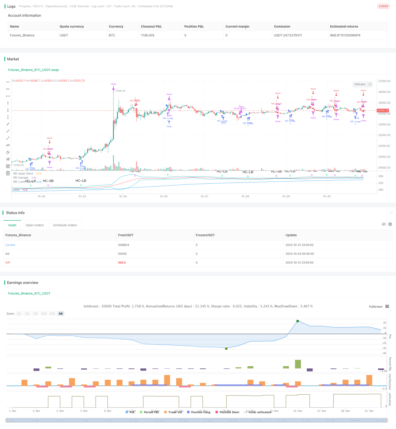
/*backtest
start: 2023-10-02 00:00:00
end: 2023-11-01 00:00:00
period: 1h
basePeriod: 15m
exchanges: [{"eid":"Futures_Binance","currency":"BTC_USDT"}]
*/

//@version=4

// This source code is subject to the terms of the Mozilla Public License 2.0 at https://mozilla.org/MPL/2.0/
// © MakeMoneyCoESTB2020

//*********************Notes for continued work***************
//3) add a Table of contents to each section of code
//4) add candle stick pattern considerations to chart
//5) add an input value for DTE range to backtest
//7) add abilit to turn on/off MACD plot
//9)
//************************************************************


//Hello my fellow investors
//After hours of reading, backtesting, and YouTube video watching
//I discovered that 200EMA, VWAP, BB, MACD, and STC 
//produce the most consistent results for investment planning.
//This strategy allows you to pick between the aforementioned indicators or layer them together.
//It works on the pricipal of:
//1) Always follow the market trend - buy/sell above/below 200EMA
//2) Follow corporate investing trends - buy/sell above/below VWAP
//3) Apply MACD check - buy--> MACD line above signal line 
// and corssover below histogram \\ sell --> MACD line below signal line 
// and crossover above histogram.
//4) Check volitility with price against BB limits upper/Sell or lower/buy
//5) When STC crosses about 10 buy and when it drops below 90 sell
//6) Exit position when stop loss is triggered or profit target is hit.  BB also provides a parameter to exit positions.

//This code is the product of many hours of hard work on the part of the greater tradingview community.  The credit goes to everyone in the community who has put code out there for the greater good.

//Happy Hunting!



//Title
// strategy("WOMBO COMBO: 100/200EMA & VWAP & MACD", shorttitle="WOMBO COMBO", default_qty_type=strategy.percent_of_equity, default_qty_value=1.5, initial_capital=10000,slippage=2, currency=currency.USD, overlay=true)

//define calculations price source
price = input(title="Price Source", defval=close)


//***************************
//Calculate 20/50/100/200EMA 
EMAlength = input(title="EMA_Length", defval=200)
EMA=ema(price, EMAlength)
//plot EMA
ColorEMA=EMAlength==200?color.blue:EMAlength==100?color.aqua:EMAlength==50?color.orange:color.red
plot(EMA, title = "EMA", color = ColorEMA)


//*****************************
//calculate VWAP
ColorVWAP = (price > vwap) ? color.lime : color.maroon
plot(vwap, title = "VWAP", color=ColorVWAP, linewidth=2)


//*****************************
//calculate MACD
//define variables for speed
fast = 12, slow = 26
//define parameters to calculate MACD
fastMA = ema(price, fast)
slowMA = ema(price, slow)
//define MACD line
macd = fastMA - slowMA
//define SIGNAL line
signal = sma(macd, 9)
//plot MACD line
//plot(macd, title = "MACD",  color=color.orange)
//plot signal line
//plot(signal, title = "Signal", color=color.purple)
//plot histogram
//define histogram colors
//col_grow_above = color.green
//col_grow_below = color.red
//col_fall_above = color.lime
//col_fall_below = color.maroon
//define histogram value
//hist = macd - signal
//plot histogram
//plot(hist, title="Histogram", style=plot.style_columns, color=(hist>=0 ? (hist[1] < hist ? col_grow_above : col_fall_above) : (hist[1] < hist ? col_grow_below : col_fall_below) ), transp=0 )


//***************************************
//Calculate Bollinger Bands
//Define BB input variables
//lengthBB = input(20, minval=1)
//multBB = input(2.0, minval=0.001, maxval=50)
lengthBB = 20
multBB = 2
//define BB average
basisBB = sma(price, lengthBB)
//define BB standar deviation
devBB = multBB * stdev(price, lengthBB)
//define BB upper and lower limits
upperBB = basisBB + devBB
lowerBB = basisBB - devBB
//Plot BB graph
ShowBB = input(title="Show BB", defval="Y", type=input.string, options=["Y", "N"])
transP = (ShowBB=="Y") ? 0 : 100
plot (upperBB, title = "BB Upper Band", color = color.aqua, transp=transP)
plot (basisBB, title = "BB Average", color = color.red, transp=transP)
plot (lowerBB, title = "BB Lower Band", color = color.aqua, transp=transP)


//*************************************************
//Calculate STC
//fastLength = input(title="MACD Fast Length", type=input.integer, defval=12)
//slowLength = input(title="MACD Slow Length", type=input.integer, defval=26)
fastLength = 23
slowLength = 50
cycleLength = input(title="Cycle Length", type=input.integer, defval=10)
//d1Length = input(title="1st %D Length", type=input.integer, defval=3)
//d2Length = input(title="2nd %D Length", type=input.integer, defval=3)
d1Length = 3
d2Length = 3
srcSTC = close

macdSTC = ema(srcSTC, fastLength) - ema(srcSTC, slowLength)
k = nz(fixnan(stoch(macdSTC, macdSTC, macdSTC, cycleLength)))
d = ema(k, d1Length)
kd = nz(fixnan(stoch(d, d, d, cycleLength)))
stc = ema(kd, d2Length)
stc := 	stc > 100 ? 100 : stc < 0 ? 0 : stc
upperSTC = input(title="Upper STC limit", defval=90)
lowerSTC = input( title="Lower STC limit", defval=10)

ma1length=35
ma1 = ema(close,ma1length)
ma2 = ema(close,EMAlength)

//STCbuy = crossover(stc, lowerSTC) and ma1>ma2 and close>ma1
//STCsell = crossunder(stc, upperSTC) and ma1<ma2 and close<ma1
STCbuy = crossover(stc, lowerSTC) 
STCsell = crossunder(stc, upperSTC) 




//*************************************************
//Candle stick patterns
//DojiSize = input(0.05, minval=0.01, title="Doji size")
//data=(abs(open - close) <= (high - low) * DojiSize)
//plotchar(data, title="Doji", text='Doji', color=color.white)

data2=(close[2] > open[2] and min(open[1], close[1]) > close[2] and open < min(open[1], close[1]) and close < open )
//plotshape(data2, title= "Evening Star", color=color.red, style=shape.arrowdown, text="Evening\nStar")

data3=(close[2] < open[2] and max(open[1], close[1]) < close[2] and open > max(open[1], close[1]) and close > open )
//plotshape(data3,  title= "Morning Star", location=location.belowbar, color=color.lime, style=shape.arrowup, text="Morning\nStar")

data4=(open[1] < close[1] and open > close[1] and high - max(open, close) >= abs(open - close) * 3 and min(close, open) - low <= abs(open - close))
//plotshape(data4, title= "Shooting Star", color=color.red, style=shape.arrowdown, text="Shooting\nStar")

data5=(((high - low)>3*(open -close)) and  ((close - low)/(.001 + high - low) > 0.6) and ((open - low)/(.001 + high - low) > 0.6))
//plotshape(data5, title= "Hammer", location=location.belowbar, color=color.white, style=shape.diamond, text="H")

data5b=(((high - low)>3*(open -close)) and  ((high - close)/(.001 + high - low) > 0.6) and ((high - open)/(.001 + high - low) > 0.6))
//plotshape(data5b, title= "Inverted Hammer", location=location.belowbar, color=color.white, style=shape.diamond, text="IH")

data6=(close[1] > open[1] and open > close and open <= close[1] and open[1] <= close and open - close < close[1] - open[1] )
//plotshape(data6, title= "Bearish Harami",  color=color.red, style=shape.arrowdown, text="Bearish\nHarami")

data7=(open[1] > close[1] and close > open and close <= open[1] and close[1] <= open and close - open < open[1] - close[1] )
//plotshape(data7,  title= "Bullish Harami", location=location.belowbar, color=color.lime, style=shape.arrowup, text="Bullish\nHarami")

data8=(close[1] > open[1] and open > close and open >= close[1] and open[1] >= close and open - close > close[1] - open[1] )
//plotshape(data8,  title= "Bearish Engulfing", color=color.red, style=shape.arrowdown, text="Bearish\nEngulfing")

data9=(open[1] > close[1] and close > open and close >= open[1] and close[1] >= open and close - open > open[1] - close[1] )
//plotshape(data9, title= "Bullish Engulfing", location=location.belowbar, color=color.lime, style=shape.arrowup, text="Bullish\nEngulfling")

upper = highest(10)[1]
data10=(close[1] < open[1] and  open < low[1] and close > close[1] + ((open[1] - close[1])/2) and close < open[1])
//plotshape(data10, title= "Piercing Line", location=location.belowbar, color=color.lime, style=shape.arrowup, text="Piercing\nLine")

lower = lowest(10)[1]
data11=(low == open and  open < lower and open < close and close > ((high[1] - low[1]) / 2) + low[1])
//plotshape(data11, title= "Bullish Belt", location=location.belowbar, color=color.lime, style=shape.arrowup, text="Bullish\nBelt")

data12=(open[1]>close[1] and open>=open[1] and close>open)
//plotshape(data12, title= "Bullish Kicker", location=location.belowbar, color=color.lime, style=shape.arrowup, text="Bullish\nKicker")

data13=(open[1]<close[1] and open<=open[1] and close<=open)
//plotshape(data13, title= "Bearish Kicker", color=color.red, style=shape.arrowdown, text="Bearish\nKicker")

data14=(((high-low>4*(open-close))and((close-low)/(.001+high-low)>=0.75)and((open-low)/(.001+high-low)>=0.75)) and high[1] < open and high[2] < open)
//plotshape(data14,  title= "Hanging Man", color=color.red, style=shape.arrowdown, text="Hanging\nMan")

data15=((close[1]>open[1])and(((close[1]+open[1])/2)>close)and(open>close)and(open>close[1])and(close>open[1])and((open-close)/(.001+(high-low))>0.6))
//plotshape(data15, title= "Dark Cloud Cover", color=color.red, style=shape.arrowdown, text="Dark\nCloudCover")




//**********Long & Short Entry Calculations***********************************
//Define countback variable
countback=input(minval=0, maxval=5, title="Price CountBack", defval=0)
//User input for what evaluations to run: EMA, VWAP, MACD, BB
EMA_Y_N=input(defval = "N", title="Run EMA", type=input.string, options=["Y", "N"])
VWAP_Y_N=input(defval = "N", title="Run VWAP", type=input.string, options=["Y", "N"])
MACD_Y_N=input(defval = "N", title="Run MACD", type=input.string, options=["Y", "N"])
BB_Y_N=input(defval = "N", title="Run BB", type=input.string, options=["Y", "N"])
STC_Y_N=input(defval = "Y", title="Run STC", type=input.string, options=["Y", "N"])
//long entry condition
dataHCLB=(iff(STC_Y_N=="Y", STCbuy, true) and iff(EMA_Y_N=="Y", price[countback]>EMA, true) and iff(VWAP_Y_N=="Y", price[countback]>vwap, true) and iff(MACD_Y_N=="Y", crossunder(signal[countback], macd[countback]), true) and iff(MACD_Y_N=="Y", macd[countback]<0, true) and iff(BB_Y_N=="Y", crossunder(price[countback], lowerBB), true))
plotshape(dataHCLB, title= "HC-LB", color=color.lime, style=shape.circle, text="HC-LB")
strategy.entry("HC-Long", strategy.long, comment="HC-Long", when = dataHCLB)
//short entry condition
dataHCSB=(iff(STC_Y_N=="Y", STCsell, true) and iff(EMA_Y_N=="Y", price[countback]<EMA, true) and iff(VWAP_Y_N=="Y", price[countback]<vwap, true) and iff(MACD_Y_N=="Y", crossunder(macd[countback], signal[countback]), true) and iff(MACD_Y_N=="Y", signal[countback]>0, true) and iff(BB_Y_N=="Y", crossover(price[countback], upperBB), true))
plotshape(dataHCSB, title= "HC-SB", color=color.fuchsia, style=shape.circle, text="HC-SB")
strategy.entry("HC-Short", strategy.short, comment="HC-Short", when=dataHCSB)




//******************Exit Conditions******************************
// Profit and Loss Exit Calculations
// User Options to Change Inputs (%)
stopPer = input(5, title='Stop Loss %', type=input.float) / 100
takePer = input(10, title='Take Profit %', type=input.float) / 100

// Determine where you've entered and in what direction
longStop = strategy.position_avg_price * (1 - stopPer)
shortStop = strategy.position_avg_price * (1 + stopPer)
shortTake = strategy.position_avg_price * (1 - takePer)
longTake = strategy.position_avg_price * (1 + takePer)

//exit position conditions and orders
if strategy.position_size > 0 or crossunder(price[countback], upperBB)
    strategy.exit(id="Close Long", stop=longStop, limit=longTake)
if strategy.position_size < 0 or crossover(price[countback], lowerBB)
    strategy.exit(id="Close Short", stop=shortStop, limit=shortTake)

Plus de

2019 FMZ - Tous les droits réservés