1. वर्ग
2. क्वांट ट्रेडिंग में ट्रेडिंग इन्फ्लेक्शन पॉइंट्स की पहचान करने के लिए मल्टी-इंडिकेटर रणनीति

क्वांट ट्रेडिंग में ट्रेडिंग इन्फ्लेक्शन पॉइंट्स की पहचान करने के लिए मल्टी-इंडिकेटर रणनीति

लेखक:चाओझांग, दिनांकः 2023-11-02 14:09:34
टैगः

---

---

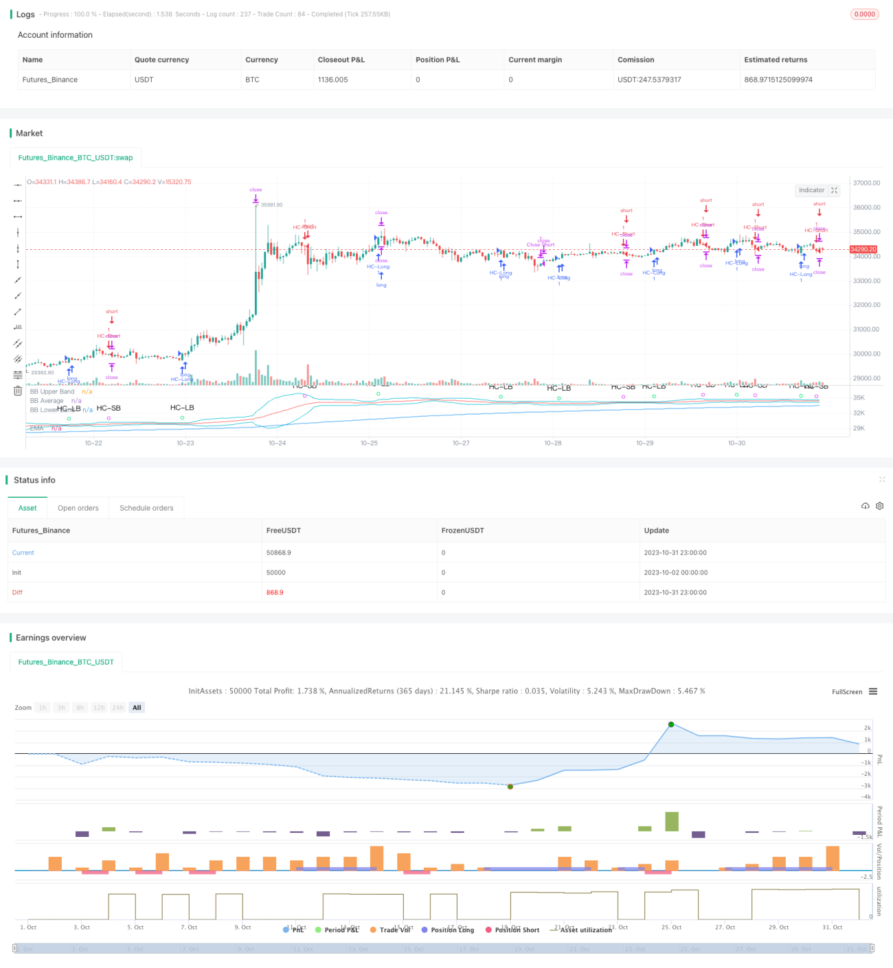
/*backtest
start: 2023-10-02 00:00:00
end: 2023-11-01 00:00:00
period: 1h
basePeriod: 15m
exchanges: [{"eid":"Futures_Binance","currency":"BTC_USDT"}]
*/

//@version=4

// This source code is subject to the terms of the Mozilla Public License 2.0 at https://mozilla.org/MPL/2.0/
// © MakeMoneyCoESTB2020

//*********************Notes for continued work***************
//3) add a Table of contents to each section of code
//4) add candle stick pattern considerations to chart
//5) add an input value for DTE range to backtest
//7) add abilit to turn on/off MACD plot
//9)
//************************************************************


//Hello my fellow investors
//After hours of reading, backtesting, and YouTube video watching
//I discovered that 200EMA, VWAP, BB, MACD, and STC 
//produce the most consistent results for investment planning.
//This strategy allows you to pick between the aforementioned indicators or layer them together.
//It works on the pricipal of:
//1) Always follow the market trend - buy/sell above/below 200EMA
//2) Follow corporate investing trends - buy/sell above/below VWAP
//3) Apply MACD check - buy--> MACD line above signal line 
// and corssover below histogram \\ sell --> MACD line below signal line 
// and crossover above histogram.
//4) Check volitility with price against BB limits upper/Sell or lower/buy
//5) When STC crosses about 10 buy and when it drops below 90 sell
//6) Exit position when stop loss is triggered or profit target is hit.  BB also provides a parameter to exit positions.

//This code is the product of many hours of hard work on the part of the greater tradingview community.  The credit goes to everyone in the community who has put code out there for the greater good.

//Happy Hunting!



//Title
// strategy("WOMBO COMBO: 100/200EMA & VWAP & MACD", shorttitle="WOMBO COMBO", default_qty_type=strategy.percent_of_equity, default_qty_value=1.5, initial_capital=10000,slippage=2, currency=currency.USD, overlay=true)

//define calculations price source
price = input(title="Price Source", defval=close)


//***************************
//Calculate 20/50/100/200EMA 
EMAlength = input(title="EMA_Length", defval=200)
EMA=ema(price, EMAlength)
//plot EMA
ColorEMA=EMAlength==200?color.blue:EMAlength==100?color.aqua:EMAlength==50?color.orange:color.red
plot(EMA, title = "EMA", color = ColorEMA)


//*****************************
//calculate VWAP
ColorVWAP = (price > vwap) ? color.lime : color.maroon
plot(vwap, title = "VWAP", color=ColorVWAP, linewidth=2)


//*****************************
//calculate MACD
//define variables for speed
fast = 12, slow = 26
//define parameters to calculate MACD
fastMA = ema(price, fast)
slowMA = ema(price, slow)
//define MACD line
macd = fastMA - slowMA
//define SIGNAL line
signal = sma(macd, 9)
//plot MACD line
//plot(macd, title = "MACD",  color=color.orange)
//plot signal line
//plot(signal, title = "Signal", color=color.purple)
//plot histogram
//define histogram colors
//col_grow_above = color.green
//col_grow_below = color.red
//col_fall_above = color.lime
//col_fall_below = color.maroon
//define histogram value
//hist = macd - signal
//plot histogram
//plot(hist, title="Histogram", style=plot.style_columns, color=(hist>=0 ? (hist[1] < hist ? col_grow_above : col_fall_above) : (hist[1] < hist ? col_grow_below : col_fall_below) ), transp=0 )


//***************************************
//Calculate Bollinger Bands
//Define BB input variables
//lengthBB = input(20, minval=1)
//multBB = input(2.0, minval=0.001, maxval=50)
lengthBB = 20
multBB = 2
//define BB average
basisBB = sma(price, lengthBB)
//define BB standar deviation
devBB = multBB * stdev(price, lengthBB)
//define BB upper and lower limits
upperBB = basisBB + devBB
lowerBB = basisBB - devBB
//Plot BB graph
ShowBB = input(title="Show BB", defval="Y", type=input.string, options=["Y", "N"])
transP = (ShowBB=="Y") ? 0 : 100
plot (upperBB, title = "BB Upper Band", color = color.aqua, transp=transP)
plot (basisBB, title = "BB Average", color = color.red, transp=transP)
plot (lowerBB, title = "BB Lower Band", color = color.aqua, transp=transP)


//*************************************************
//Calculate STC
//fastLength = input(title="MACD Fast Length", type=input.integer, defval=12)
//slowLength = input(title="MACD Slow Length", type=input.integer, defval=26)
fastLength = 23
slowLength = 50
cycleLength = input(title="Cycle Length", type=input.integer, defval=10)
//d1Length = input(title="1st %D Length", type=input.integer, defval=3)
//d2Length = input(title="2nd %D Length", type=input.integer, defval=3)
d1Length = 3
d2Length = 3
srcSTC = close

macdSTC = ema(srcSTC, fastLength) - ema(srcSTC, slowLength)
k = nz(fixnan(stoch(macdSTC, macdSTC, macdSTC, cycleLength)))
d = ema(k, d1Length)
kd = nz(fixnan(stoch(d, d, d, cycleLength)))
stc = ema(kd, d2Length)
stc := 	stc > 100 ? 100 : stc < 0 ? 0 : stc
upperSTC = input(title="Upper STC limit", defval=90)
lowerSTC = input( title="Lower STC limit", defval=10)

ma1length=35
ma1 = ema(close,ma1length)
ma2 = ema(close,EMAlength)

//STCbuy = crossover(stc, lowerSTC) and ma1>ma2 and close>ma1
//STCsell = crossunder(stc, upperSTC) and ma1<ma2 and close<ma1
STCbuy = crossover(stc, lowerSTC) 
STCsell = crossunder(stc, upperSTC) 




//*************************************************
//Candle stick patterns
//DojiSize = input(0.05, minval=0.01, title="Doji size")
//data=(abs(open - close) <= (high - low) * DojiSize)
//plotchar(data, title="Doji", text='Doji', color=color.white)

data2=(close[2] > open[2] and min(open[1], close[1]) > close[2] and open < min(open[1], close[1]) and close < open )
//plotshape(data2, title= "Evening Star", color=color.red, style=shape.arrowdown, text="Evening\nStar")

data3=(close[2] < open[2] and max(open[1], close[1]) < close[2] and open > max(open[1], close[1]) and close > open )
//plotshape(data3,  title= "Morning Star", location=location.belowbar, color=color.lime, style=shape.arrowup, text="Morning\nStar")

data4=(open[1] < close[1] and open > close[1] and high - max(open, close) >= abs(open - close) * 3 and min(close, open) - low <= abs(open - close))
//plotshape(data4, title= "Shooting Star", color=color.red, style=shape.arrowdown, text="Shooting\nStar")

data5=(((high - low)>3*(open -close)) and  ((close - low)/(.001 + high - low) > 0.6) and ((open - low)/(.001 + high - low) > 0.6))
//plotshape(data5, title= "Hammer", location=location.belowbar, color=color.white, style=shape.diamond, text="H")

data5b=(((high - low)>3*(open -close)) and  ((high - close)/(.001 + high - low) > 0.6) and ((high - open)/(.001 + high - low) > 0.6))
//plotshape(data5b, title= "Inverted Hammer", location=location.belowbar, color=color.white, style=shape.diamond, text="IH")

data6=(close[1] > open[1] and open > close and open <= close[1] and open[1] <= close and open - close < close[1] - open[1] )
//plotshape(data6, title= "Bearish Harami",  color=color.red, style=shape.arrowdown, text="Bearish\nHarami")

data7=(open[1] > close[1] and close > open and close <= open[1] and close[1] <= open and close - open < open[1] - close[1] )
//plotshape(data7,  title= "Bullish Harami", location=location.belowbar, color=color.lime, style=shape.arrowup, text="Bullish\nHarami")

data8=(close[1] > open[1] and open > close and open >= close[1] and open[1] >= close and open - close > close[1] - open[1] )
//plotshape(data8,  title= "Bearish Engulfing", color=color.red, style=shape.arrowdown, text="Bearish\nEngulfing")

data9=(open[1] > close[1] and close > open and close >= open[1] and close[1] >= open and close - open > open[1] - close[1] )
//plotshape(data9, title= "Bullish Engulfing", location=location.belowbar, color=color.lime, style=shape.arrowup, text="Bullish\nEngulfling")

upper = highest(10)[1]
data10=(close[1] < open[1] and  open < low[1] and close > close[1] + ((open[1] - close[1])/2) and close < open[1])
//plotshape(data10, title= "Piercing Line", location=location.belowbar, color=color.lime, style=shape.arrowup, text="Piercing\nLine")

lower = lowest(10)[1]
data11=(low == open and  open < lower and open < close and close > ((high[1] - low[1]) / 2) + low[1])
//plotshape(data11, title= "Bullish Belt", location=location.belowbar, color=color.lime, style=shape.arrowup, text="Bullish\nBelt")

data12=(open[1]>close[1] and open>=open[1] and close>open)
//plotshape(data12, title= "Bullish Kicker", location=location.belowbar, color=color.lime, style=shape.arrowup, text="Bullish\nKicker")

data13=(open[1]<close[1] and open<=open[1] and close<=open)
//plotshape(data13, title= "Bearish Kicker", color=color.red, style=shape.arrowdown, text="Bearish\nKicker")

data14=(((high-low>4*(open-close))and((close-low)/(.001+high-low)>=0.75)and((open-low)/(.001+high-low)>=0.75)) and high[1] < open and high[2] < open)
//plotshape(data14,  title= "Hanging Man", color=color.red, style=shape.arrowdown, text="Hanging\nMan")

data15=((close[1]>open[1])and(((close[1]+open[1])/2)>close)and(open>close)and(open>close[1])and(close>open[1])and((open-close)/(.001+(high-low))>0.6))
//plotshape(data15, title= "Dark Cloud Cover", color=color.red, style=shape.arrowdown, text="Dark\nCloudCover")




//**********Long & Short Entry Calculations***********************************
//Define countback variable
countback=input(minval=0, maxval=5, title="Price CountBack", defval=0)
//User input for what evaluations to run: EMA, VWAP, MACD, BB
EMA_Y_N=input(defval = "N", title="Run EMA", type=input.string, options=["Y", "N"])
VWAP_Y_N=input(defval = "N", title="Run VWAP", type=input.string, options=["Y", "N"])
MACD_Y_N=input(defval = "N", title="Run MACD", type=input.string, options=["Y", "N"])
BB_Y_N=input(defval = "N", title="Run BB", type=input.string, options=["Y", "N"])
STC_Y_N=input(defval = "Y", title="Run STC", type=input.string, options=["Y", "N"])
//long entry condition
dataHCLB=(iff(STC_Y_N=="Y", STCbuy, true) and iff(EMA_Y_N=="Y", price[countback]>EMA, true) and iff(VWAP_Y_N=="Y", price[countback]>vwap, true) and iff(MACD_Y_N=="Y", crossunder(signal[countback], macd[countback]), true) and iff(MACD_Y_N=="Y", macd[countback]<0, true) and iff(BB_Y_N=="Y", crossunder(price[countback], lowerBB), true))
plotshape(dataHCLB, title= "HC-LB", color=color.lime, style=shape.circle, text="HC-LB")
strategy.entry("HC-Long", strategy.long, comment="HC-Long", when = dataHCLB)
//short entry condition
dataHCSB=(iff(STC_Y_N=="Y", STCsell, true) and iff(EMA_Y_N=="Y", price[countback]<EMA, true) and iff(VWAP_Y_N=="Y", price[countback]<vwap, true) and iff(MACD_Y_N=="Y", crossunder(macd[countback], signal[countback]), true) and iff(MACD_Y_N=="Y", signal[countback]>0, true) and iff(BB_Y_N=="Y", crossover(price[countback], upperBB), true))
plotshape(dataHCSB, title= "HC-SB", color=color.fuchsia, style=shape.circle, text="HC-SB")
strategy.entry("HC-Short", strategy.short, comment="HC-Short", when=dataHCSB)




//******************Exit Conditions******************************
// Profit and Loss Exit Calculations
// User Options to Change Inputs (%)
stopPer = input(5, title='Stop Loss %', type=input.float) / 100
takePer = input(10, title='Take Profit %', type=input.float) / 100

// Determine where you've entered and in what direction
longStop = strategy.position_avg_price * (1 - stopPer)
shortStop = strategy.position_avg_price * (1 + stopPer)
shortTake = strategy.position_avg_price * (1 - takePer)
longTake = strategy.position_avg_price * (1 + takePer)

//exit position conditions and orders
if strategy.position_size > 0 or crossunder(price[countback], upperBB)
    strategy.exit(id="Close Long", stop=longStop, limit=longTake)
if strategy.position_size < 0 or crossover(price[countback], lowerBB)
    strategy.exit(id="Close Short", stop=shortStop, limit=shortTake)

---

• आरएसआई डेयरडेविल स्क्वाड्रन संलयन रणनीति
• ट्रिपल मूविंग एवरेज ट्रेडिंग रणनीति
• प्राइम नंबर ऑसिलेटर ट्रेडिंग रणनीति
• गति का ब्रेकअप रणनीति की पहचान करता है
• ट्रिपल आरएसआई एक्सट्रीम ट्रेडिंग रणनीति
• गोल्डन क्रॉस केल्टनर चैनल ट्रेंड रणनीति का पालन करना
• मासिक उद्घाटन लंबी और महीने के अंत में समापन रणनीति
• दोहरी चलती औसत क्रॉसओवर ट्रेडिंग रणनीति
• ट्रेंड लाइन ट्रेडिंग रणनीति
• स्टोकैस्टिक आरएसआई और वॉल्यूम आधारित ट्रेडिंग रणनीति
• एटीआर ट्रैलिंग स्टॉप रणनीति (केवल लंबी)
• ट्रेंड ट्रैकिंग पर आधारित गति व्यापार रणनीति स्टॉप लॉस
• दोहरे दबाव की मात्रात्मक व्यापारिक रणनीति
• राक्षस कंपनी के वीवीसीएन राक्षस रोबोट संदेश भेजते हैं
• ब्रेकआउट ट्रेंड फॉलोअर V2
• चलती औसत क्रॉसओवर रणनीति के बाद की प्रवृत्ति
• गति ब्रेकआउट मूविंग एवरेज ट्रेडिंग रणनीति
• हुल मूविंग एवरेज और कालमैन फिल्टर आधारित ट्रेंड ट्रैकिंग रणनीति
• गोल्डन क्रॉस ट्रेंड रणनीति का पालन करना
• सिग्नल-टू-शोर अनुपात अनुकूलन कॉम्बो रणनीति