판다와 함께 파이썬에서 이동 평균 크로스오버를 백테스트하는 것

이 기사에서는 우리가 도입한 기계를 사용하여 실제 전략, 즉 AAPL에 대한 이동 평균 크로스오버에 대한 연구를 수행 할 것입니다.

이동 평균 크로스오버 전략

이동 평균 크로스오버 기법은 매우 잘 알려진 단순화 된 모멘텀 전략입니다. 양적 거래의 "안녕하세요 세계" 예로 종종 간주됩니다.

여기서 설명한 전략은 길게만 사용된다. 특정 시간대에서 서로 다른 룩백 기간을 가진 두 개의 별도의 간단한 이동 평균 필터가 생성된다. 짧은 룩백 이동 평균이 더 긴 룩백 이동 평균을 초과할 때 자산 구매 신호가 발생한다. 더 긴 평균이 나중에 짧은 평균을 초과하면 자산이 다시 판매된다. 시간대가 강한 트렌드의 기간에 들어가서 천천히 트렌드를 역전할 때 전략은 잘 작동한다.

이 예제에서, 나는 100일 짧은 룩백과 400일 긴 룩백과 함께 Apple, Inc. (AAPL) 를 시간 계열로 선택했습니다. 이것은 zipline 알고리즘 거래 라이브러리가 제공하는 예입니다. 따라서 우리가 우리 자신의 백테스터를 구현하고 싶다면 zipline의 결과와 일치하는지 확인해야합니다.

시행

여기 이전 튜토리얼을 따르도록 하십시오. 이 튜토리얼은 백테스터의 초기 객체 계층이 어떻게 구성되는지 설명합니다. 그렇지 않으면 아래 코드가 작동하지 않습니다. 이 특정 구현을 위해 다음 라이브러리를 사용했습니다.

• 파이썬 - 2.7.3
• 수 - 1.8.0
• 판다 - 0.12.0
• matplotlib - 1.1.0

ma_cross.py의 구현은backtest.py첫 번째 단계는 필요한 모듈과 객체를 수입하는 것입니다:

# ma_cross.py

import datetime
import matplotlib.pyplot as plt
import numpy as np
import pandas as pd

from pandas.io.data import DataReader
from backtest import Strategy, Portfolio

이전 튜토리얼에서와 마찬가지로 우리는 AAPL의 이동 평균이 서로 횡단할 때 신호를 생성하는 방법에 대한 모든 세부 사항을 포함하는 MovingAverageCrossStrategy를 생성하기 위해 전략 추상 기본 클래스를 하급할 것입니다.

이 객체는 동작할 수 있는 short_window와 long_window를 필요로 합니다. 값은 zipline의 주요 예제에서 사용된 동일한 매개 변수인 각각 100일과 400일의 기본값으로 설정되었습니다.

이동 평균은 AAPL 주식의 막대기[Close] 닫기 가격에 있는 panda rolling_mean 함수를 사용하여 생성된다. 개별 이동 평균이 구성된 후에는 짧은 이동 평균이 긴 이동 평균보다 크거나 다른 경우 0.0이 될 때 열을 1.0로 설정하여 신호 시리즈를 생성한다. 이로부터 포지션 오더를 생성하여 거래 신호를 나타낼 수 있다.

# ma_cross.py

class MovingAverageCrossStrategy(Strategy):
    """    
    Requires:
    symbol - A stock symbol on which to form a strategy on.
    bars - A DataFrame of bars for the above symbol.
    short_window - Lookback period for short moving average.
    long_window - Lookback period for long moving average."""

    def __init__(self, symbol, bars, short_window=100, long_window=400):
        self.symbol = symbol
        self.bars = bars

        self.short_window = short_window
        self.long_window = long_window

    def generate_signals(self):
        """Returns the DataFrame of symbols containing the signals
        to go long, short or hold (1, -1 or 0)."""
        signals = pd.DataFrame(index=self.bars.index)
        signals['signal'] = 0.0

        # Create the set of short and long simple moving averages over the 
        # respective periods
        signals['short_mavg'] = pd.rolling_mean(bars['Close'], self.short_window, min_periods=1)
        signals['long_mavg'] = pd.rolling_mean(bars['Close'], self.long_window, min_periods=1)

        # Create a 'signal' (invested or not invested) when the short moving average crosses the long
        # moving average, but only for the period greater than the shortest moving average window
        signals['signal'][self.short_window:] = np.where(signals['short_mavg'][self.short_window:] 
            > signals['long_mavg'][self.short_window:], 1.0, 0.0)   

        # Take the difference of the signals in order to generate actual trading orders
        signals['positions'] = signals['signal'].diff()   

        return signals

MarketOnClose포트폴리오는 포트폴리오에서 하위 분류됩니다.backtest.py포트폴리오 객체가 어떻게 정의되는지에 대한 자세한 내용은 이전 튜토리얼을 참조하십시오. 전면성을 위해 코드를 남겨두고 이 튜토리얼을 자체적으로 유지하기 위해:

# ma_cross.py

class MarketOnClosePortfolio(Portfolio):
    """Encapsulates the notion of a portfolio of positions based
    on a set of signals as provided by a Strategy.

    Requires:
    symbol - A stock symbol which forms the basis of the portfolio.
    bars - A DataFrame of bars for a symbol set.
    signals - A pandas DataFrame of signals (1, 0, -1) for each symbol.
    initial_capital - The amount in cash at the start of the portfolio."""

    def __init__(self, symbol, bars, signals, initial_capital=100000.0):
        self.symbol = symbol        
        self.bars = bars
        self.signals = signals
        self.initial_capital = float(initial_capital)
        self.positions = self.generate_positions()
        
    def generate_positions(self):
        positions = pd.DataFrame(index=signals.index).fillna(0.0)
        positions[self.symbol] = 100*signals['signal']   # This strategy buys 100 shares
        return positions
                    
    def backtest_portfolio(self):
        portfolio = self.positions*self.bars['Close']
        pos_diff = self.positions.diff()

        portfolio['holdings'] = (self.positions*self.bars['Close']).sum(axis=1)
        portfolio['cash'] = self.initial_capital - (pos_diff*self.bars['Close']).sum(axis=1).cumsum()

        portfolio['total'] = portfolio['cash'] + portfolio['holdings']
        portfolio['returns'] = portfolio['total'].pct_change()
        return portfolio

이제 이동 평균 크로스 전략과 마켓 온 클로즈 포트폴리오 클래스가 정의되었습니다.주요기능의 모든 기능을 묶는 기능을 호출 할 것입니다. 또한 전략의 성능은 주식 곡선의 그래프를 통해 검토됩니다.

판다 데이터 리더 객체는 1990년 1월 1일부터 2002년 1월 1일까지 AAPL 주식의 OHLCV 가격을 다운로드합니다. 이 시점에서는 데이터 프레임 신호가 롱-온리 신호를 생성하기 위해 생성됩니다. 그 후 포트폴리오는 100,000 USD의 초기 자본 기반으로 생성되며 수익은 주식 곡선에서 계산됩니다.

마지막 단계는 matplotlib을 사용하여 AAPL 가격의 2자리 그래프를 그리는 것입니다. 이동 평균과 구매/판매 신호, 그리고 동일한 구매/판매 신호로 주식 곡선이 덮여 있습니다. 그래핑 코드는 zipline 구현 예제에서 가져옵니다.

# ma_cross.py

if __name__ == "__main__":
    # Obtain daily bars of AAPL from Yahoo Finance for the period
    # 1st Jan 1990 to 1st Jan 2002 - This is an example from ZipLine
    symbol = 'AAPL'
    bars = DataReader(symbol, "yahoo", datetime.datetime(1990,1,1), datetime.datetime(2002,1,1))

    # Create a Moving Average Cross Strategy instance with a short moving
    # average window of 100 days and a long window of 400 days
    mac = MovingAverageCrossStrategy(symbol, bars, short_window=100, long_window=400)
    signals = mac.generate_signals()

    # Create a portfolio of AAPL, with $100,000 initial capital
    portfolio = MarketOnClosePortfolio(symbol, bars, signals, initial_capital=100000.0)
    returns = portfolio.backtest_portfolio()

    # Plot two charts to assess trades and equity curve
    fig = plt.figure()
    fig.patch.set_facecolor('white')     # Set the outer colour to white
    ax1 = fig.add_subplot(211,  ylabel='Price in $')
    
    # Plot the AAPL closing price overlaid with the moving averages
    bars['Close'].plot(ax=ax1, color='r', lw=2.)
    signals[['short_mavg', 'long_mavg']].plot(ax=ax1, lw=2.)

    # Plot the "buy" trades against AAPL
    ax1.plot(signals.ix[signals.positions == 1.0].index, 
             signals.short_mavg[signals.positions == 1.0],
             '^', markersize=10, color='m')

    # Plot the "sell" trades against AAPL
    ax1.plot(signals.ix[signals.positions == -1.0].index, 
             signals.short_mavg[signals.positions == -1.0],
             'v', markersize=10, color='k')

    # Plot the equity curve in dollars
    ax2 = fig.add_subplot(212, ylabel='Portfolio value in $')
    returns['total'].plot(ax=ax2, lw=2.)

    # Plot the "buy" and "sell" trades against the equity curve
    ax2.plot(returns.ix[signals.positions == 1.0].index, 
             returns.total[signals.positions == 1.0],
             '^', markersize=10, color='m')
    ax2.plot(returns.ix[signals.positions == -1.0].index, 
             returns.total[signals.positions == -1.0],
             'v', markersize=10, color='k')

    # Plot the figure
    fig.show()

코드의 그래픽 출력은 다음과 같습니다. 저는 IPython %paste 명령어를 사용하여 Ubuntu에서 IPython 콘솔에 직접 넣었습니다. 그래픽 출력은 여전히 볼 수 있습니다. 분홍색의 상승은 주식을 구매하는 것을 나타냅니다. 검은색의 하락은 다시 판매하는 것을 나타냅니다.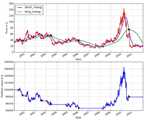1990-01-01에서 2002-01-01까지 AAPL 이동 평균 크로스오버 성능

보시다시피 전략은 기간 동안 돈을 잃어 버립니다. 5 개의 왕복 거래로. 이 기간 동안 AAPL의 행동이 가벼운 하락 추세를 보이며 1998 년부터 상당한 상승을 거듭했기 때문에 놀라운 일이 아닙니다. 이동 평균 신호의 리크백 기간은 상당히 크며 이것이 최종 거래의 이익에 영향을 미쳤으며, 그렇지 않으면 전략을 수익성있게 만들 수 있습니다.

다음 기사에서는 성능을 분석하는 더 정교한 방법을 만들 것이며 개별 이동 평균 신호의 룩백 기간을 최적화하는 방법을 설명 할 것입니다.